


面向近红外光谱定量分析的深度学习建模与模型迁移
[傅鹏有1, 2  , 文岳
, 文岳2 , 张雨柯3 , 李灵巧1, * , 杨辉华1, 2, * ]
, 文岳, 杨辉华]
|
|


近红外光谱分析技术依赖于表征光谱向量和预测目标之间关系的化学计量学方法。 然而, 样品的光谱由信号和各种噪声组成, 传统化学计量学方法较难直接提取光谱的有效特征, 并为复杂的预测任务建立具有较强泛用性的校正模型。 进一步地, 受限于仪器间的差异, 在一台仪器上建立的模型应用于另一台仪器时, 难以取得相同的定量分析结果。 为此, 提出了一种基于卷积神经网络和迁移学习的定量分析建模及模型传递方案, 以提高模型在单仪器和跨仪器上的预测性能。 在卷积神经网络的基础上, 一种结合多尺度特征融合和残差结构, 名为MSRCNN的先进模型被设计, 并在主仪器上展现了卓越的预测能力。 然后, 设计了四种的基于fine-tune模型迁移策略, 将在主仪器上建立的MSRCNN模型迁移到从仪器。 在药品和小麦的公开数据集上的实验结果表明, MSRCNN在主仪器上的RMSE和 R2分别为2.587, 0.981和0.309, 0.977, 优于PLS, SVM和CNN。 在利用30个从仪器的样本微调主仪器建立的模型后, 迁移MSRCNN中的卷积层和全连接层的方案取得了最好效果, 其RMSE和R2可分别达到2.289, 0.982和0.379, 0.965。 增加参与模型微调的从仪器样本, 可进一步提高性能。
Biography: FU Peng-you, (1998—), Master's degree reading, School of Computer Science and Information Security, Guilin University of Electronic Technology e-mail: 20032201004@mails.guet.edu.cn
Near-infrared spectroscoqy analysis technologyrelies on Chemometric methods that characterize the relationships between the spectral matrix and the chemical or physical properties. However, the samples' spectra are composed of signals and various noises. It is difficult for traditional Chemometric methods to extract the effective features of the spectra and establish a calibration model with strong generative performance for a complex assay. Furthermore, the same quantitative analysis results cannot be achieved when the calibration model established on one instrument is applied to another because of the differences between the instruments. Hence, this paper presents a quantitative analysis modeling and model transfer frameworkbased on convolution neural networks and transfer learning to improve model prediction performance on one instrument and across the instrument. An advanced model named MSRCNN is presented based on a convolutional neural network, which integrates multi-scale feature fusion and residual structure and shows outstanding model generalization performance on the master instrument. Then, four transfer learning methods based on fine-tuning are proposed to transfer the MSRCNN established on the master instrument to the slave instrument. The experimental results on open accessed datasets of drug and wheat show that the RMSE and R2 of MSRCNN on the master instrument are 2.587, 0.981, and 0.309, 0.977, respectively, which outperforms PLS, SVM, and CNN. Byusing 30 slave instrument samples, the transfer of the convolutional layer and fully connected layer in the MSRCNN model is the most effective among the four fine-tune methods, with RMSE and R2 2.289, 0.982, and 0.379, 0.965, respectively. The performance can be further improved by increasing the sample of slave instruments that participated in model transferring.
Near-infrared analysis technology is widely used in agriculture, food, the environment, the chemical industry, and other fields with the characteristics of non-destructive, pollution-free, and fast detection[1, 2, 3, 4]. However, its application depends on the Chemometric method that characterizes the relationship between the spectral vector and the chemical or physical properties. Traditional Chemometrics methods (PLS, SVM, etc.) performs pretty well under the simple situation. But it is difficult to extract effective information directly from spectra with complex noises, so they often need the aid of pre-processing and wavelength selection algorithms with prior knowledge[5, 6]. In addition, due to the limitations of existing manufacturing techniques and the aging of instruments, there are also differences among the same type of NIR spectrometer manufactured by the same manufacturer, which makes it difficult to generalize the calibration model with good effect established on one instrument to another instrument[7, 8, 9, 10, 11]. This degrades the generalization of the calibration model and the application of near-infrared analysis technology. Therefore, extracting spectral features, establishing models with good predictive capabilities, improving model generalization, and enabling models to be shared among different types of instruments have always been the focus of Chemometrics research[12, 13, 14, 15].
As one of the classical deep learning methods, the convolution neural network has shown great potential in spectral feature extraction and has been applied to qualitative and quantitative analysis. Acquarelli et al.[16] introduced convolutional neural networks into spectrum analysis, and the results are superior to the classical PLS-LDA and KNN algorithms on multiple data sets. Zhang et al.[17] draw on the Inception structure, the Deep Spectra model based on the idea of multi-scale fusion has achieved better results than PLS and SVR, and the experiments show that it is easier to obtain effective features of spectra by increasing the network width. Dong et al.[18] and Jiang et al.[19] introduce a residual mechanism to construct a deep Resnet network, which is used to trace the origin of Panax notoginseng and tobacco respectively, and further improve the classification accuracy compared with common convolution network and GA-SVM. Although CNN has shown excellent performance in prediction ability, it is mainly a nonlinear convolution structure with multi-layer stacking. However, the traditional model transfer method only applies to PLS and other multivariate linear models and cannot be applied to the model transfer of CNN networks[20, 21, 22].
Transfer learning refers to transferring the trained data domain model to another related but different data domain by using the similarity of data distribution among different domains[23]. Although it has been widely used in image processing, natural language processing and other fields[24, 25, 26, 27], the research in the spectral analysis is still in the initial stage. Li et al.[28] constructed a convolution network model on a single class of drugs, and then used transfer learning to transfer the calibration model to other classes to realize the identification of multiple classes of drugs by a single model. Mishra et al.[29] Using transfer learning to transfer a convolution network built on many samples to a small number of sample data sets overcomes the data sensitivity of a deep learning model. Mishra et al.[30] also tried to transfer convolutional network models between different instruments based on two transfer learning methods, and the experimental results on the two data sets showed that it could effectively improve the model's versatility. Previous studies have shown that the introduction of transfer learning can realize the transfer of convolutional models between similar data sets and can be used to alleviate the differences between measuring instruments.
Because of this, this paper proposes a spectral modelling and model transfer method based on convolution neural network and transfer learning: First, based on ordinary convolutional networks, multi-scale fusion and residual mechanisms are introduced to construct a convolution model with better predictive ability and generalization. Then, the model built on the master instrument is transferred to the slave instrument using the cross-domain knowledge-sharing ability of transfer learning, and the model is recalibrated by using fewer data samples of transformation sets. At the same time, in order to further understand and apply transfer learning, this paper also designed four different model transfer methods to compare and discuss the impact of different transfer strategies on model transfer performance. The source code is available at https://github.com/FuSiry/DeepNirs-cnn-transfer for academic use only.
1.1.1 Pharmaceutical data set
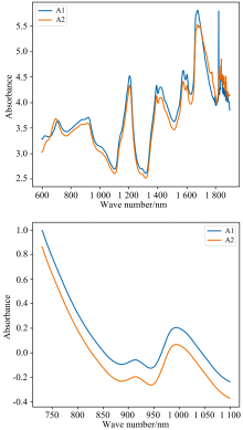
The first data set comes from the open-source data set released by IDRC 2002. The data consists of 655 tablet samples, with a wavelength range of 600 to 1 898 nm, an interval of 2 nm, and a total of 649 sample points. It is measured by two instruments (A1, A2). The original spectral difference of a sample of A1 and A2 is shown in Fig.1(a). The data can be downloaded from http://www.eigenvector.com/data/tablets/index.htm.
 | Fig.1 Spectrum of the same sample under different instruments |
1.1.2 Wheat data set
The second data set is derived from the open-source data set released by IDRC 2016 and consists of 248 wheat samples measured by three manufacturers' instruments. To facilitate comparison with existing studies, A manufacturer's A1 and A2 instruments were selected to measure the wheat spectra, ranging in wavelength from 730 to 1 100 nm, with intervals of 0.5 nm and a total of 741 data points. The spectral differences between a sample of A1 and A2 are shown in Fig.1(b). The data can be downloaded from http://www.idr-chambersburg.org/content.aspx?page_id=22& club_id=409746& module_id=19111.
1.2.1 Inception structure
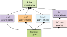
Prior knowledge in the fields of image and speech shows that widening or deepening the network is one of the methods to effectively improve the feature extraction ability of the model[31, 32]. Previous studies in the NIR field have also shown that different convolution kernels with different sizes extract different spectral information, and that inappropriate convolution kernel will lose the most important spectral crest information[33]. In order to improve the receptive field of the model and obtain information on different smoothness degrees, the Inception structure is introduced, as shown in Fig.2.
 | Fig.2 Improved inception structure |
m1, m2, m3 represent large, medium, and small convolution respectively.Large-scale convolution can learn sparse information, while small-scale convolution can easily learn non-sparse information. Convolution of different scales can increase the adaptability of the network to the spectrum, obtain spectral information with different flatness, and then improve the feature extraction ability.
1.2.2 Resnet structure
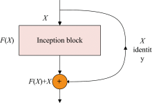
The stacking of network layers will make the extracted feature levels richer. But by simply deepening the number of network layers, under the chain rule, the gradient will continue to multiply, and eventually, the problem of gradient disappearance and explosion will occur. For this reason, a residual mechanism is added based on Inception, as shown in Fig.3.
 | Fig.3 Residual mechanism |
x denotes the input and is the output of theinput after the convolutionlayer. Therefore, during the back propagation process, the gradient information propagated by F(x) and x can be accepted simultaneously. The updated signal can still be obtained through branch x even if the network is too deep.As a result, the loss of gradients can be successfully inhibited.
1.2.3 The proposed network structure
The improved convolutional network modelin this paper is shown in Fig.4, where the Inception structure aod residual mechanism are introduced after the first layer of ordinary convolution to construct 2 Inception-Resnet convolutional layers.
 | Fig.4 The convolutional neural network structure used in this study |
After each convolution, the ReLu activation function increase the nonlinear representation and performs BN (Batch Normalization, BN). In addition, a global average!adaptive pooling layer is added after the convolution layer to reduce the network parameters, adapt to different spectrum wavelength, and avoid overfitting.
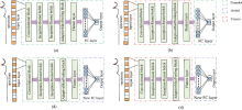
Although there are variances between instruments of different models, the challenge of forecasting the spectsum is important. As a result, an attempt is made to introduce transfer learning based on the proposed model in order to achieve model transfer between different instruments. The convolutional layer in CNN is responsible for translating the original data to the hidden feature space and for feature extraction. The fully connected layer's essence is to linearly transform one feature space to another, equivalent to feature weighting. The sensitivity of various instrument models to feature extraction and feature weighting is unknown. Considering this, four distinct transfer methods, as depicted in Fig.5, were developed to investigate the effect of transfer strategies for various network structures on model transfer performance.
 | Fig.5 Four different model transfer methods |
The network on the source domain is shown in Fig.4. In the first method, all layers and parameters of the network trained by the master instrument are transferred, the parameters of any layer are not frozen, and the whole network is fine-tunable for updating, as in Fig.5(a).The second method still transfer all layers and parameters, but freezes the parameters of the convolutional layer, and only the parameters of the fully connected layer can be updated, as in Fig.5(b). In the third method, only the convolutional layers and parameters of the network are transferred, the fully connected layers are rebuilt and initialized, and all of them can be updated after the transfer, as in Fig.5(c). In the fourth method, only the convolutional layer is transferred, the parameters are frozen, and the fully connected layer is rebuilt and initialized, as in Fig.5(d).
1.4.1 Experimental Environment
The experiments were done on an AMD Ryzen 5 3600 6-Core CPU, and NVIDIA GeForce RTX 2060 Super GPU. All models were implemented in Python as the coding tool based on the Pytorch framework and the Scikit-learn library.
1.4.2 Comparative experimental
Classical Chemometric methods PLS, SVR, ordinary convolutional neural network (CNN), and the modified multi-scale fused residual convolutional network (MSRCNN) are used to compare the feature extraction ability. PLS and SVR are implemented using Scikit-learn. The structure of the ordinary convolutional network is similar to the network shown in Fig.4, only the Inception-Resnet block is replaced with ordinary convolution, and the rest is left unchanged.
1.4.3 Model pre-training and transfer
The model is built and trained on the master instrument, with the batchsize set to 128 for the drug dataset and 16 for the wheat data. The initial learning rateon both datasets is set to 0.01, and the maximum training eopch is set to 600, both using the Adam optimizer. To balance the training time and training effect, a learning rate decay strategy is introduced, in which the learning rate is changed to half of the current value if the loss of the calibration set does not decrease within 20 training cycles. In addition, the training process is monitored using an early stop, and the loss of the test set is stopped early if it does not decrease within 60 training cycles to prevent overfitting.
The training model built on the master instrumentwas transferred to the slave instrument, and the initial learning rate was set to 0.001 on both drug datasets and 0.01 on the wheat data. To reduce the gradient descent rate on the drug, the SGD optimizer was used on the drug data, while the Adam optimizer was used on the wheat dataset. The maximum training eopch was set to 600 for both datasets, and both used the learning decay and earlystop strategies, which were the same as those set during pre-training.
As shown in formulas 1 and 2, the model's evaluation indicators are the Root Mean Squared Error (RMSE) and the coefficient of determination (R2). The RMSE measures the difference between the predicted and true values, and R2 is used to assess the degree of fit of the regression model.
Where, yi and
2.1.1 Model prediction performance
The A1 instrument is used as the master instrument. 14 abnormal samples are deleted. The 451 samples originally marked as the test set are used as the calibration set, and the two data sets originally marked as the calibration set and the validation set are combined into one test set, resulting in a total of 190 samples. In order to improve the training speed, the data is pre-processed by standardization in advance. Then 4 methods, including PLS, SVR, CNN, and MSRCNN, are used to establish calibration models respectively. The prediction results of the A1 validation set and A2 by these calibration models are shown in Table 1.
| Table 1 A1 establishes a model to directly predict the results of A1 and A2 |
The convolution model shows stronger predictive performance than the classical Chemometric method. At the same time, the prediction ability of the improved MSRCNN model in this study is further improved than that of the ordinary CNN, and the best results are obtained. The RMSE and R2 reach 2.587 and 0.981, respectively, verifying the effectiveness of introducting multi-scale fusion and residual structure. However, whether it is a convolutional network, a PLS, or an SVR model, A2 has a poor direct prediction effect. Especially in the PLS method, R2 is directly negative, and it is impossible to fit the spectrum collected by the A2 instrument. Although MSRCNN is the best method in the comparison, R2 reaches 0.939 and is still available, but the model's prediction performance is much lower than when using A1. This means that the model established on A1 directly applying to the spectrum of A2 would result in larger prediction errors.
2.1.2 Modeltransfer
The convolutional network model established on the master instrument A1 is transferred to the slave instrument A2 using the four transfer methods described in section 2.3. To compare to existing methods, 30 samples from the A2 data set are chosen at random as the training set, and the transfer model is fine-tuned. The results of using the fine-tuned model to predict the remaining 609 samples are shown in Table 2.
| Table 2 Prediction results of the convolution model under four transfer modes |
Every transfer strategy with different network structures can improve the model's prediction results in the drug set. However, the MSRCNN model predicts better than the CNN model under different transfer methods, indicating that the model with better predictions before the transfer has better prediction results after the transfer. The MSRCNN model has the best prediction results through the second type of transfer method. Its RMSE and R2 reach 2.289 and 0.982 respectively, which are better than the current methods[20, 21, 22, 30]. This verifies the effectiveness of the method in this paper.
Furthermore, it is easy to discover that the transfer methods of various network structures have a greater impact on prediction performance. When the first and third transfer methods are compared to the second and fourth transfer methods, the updated convolutional layer and the fixed convolutional layer have little effect on transfer performance. However, when comparing the first and second types of transfer with the third and fourth types, it is clear that whether the fully connected layer is transferred has a greater impact on model transfer performance. For this reason, the MSRCNN model with better prediction performance is selected as the object. The prediction results of 609 prediction samples are shown in Fig.6. Red and yellow points respectively represent the prediction points before and after the model is transferred, and the blue line represents the reference value. The closer to the blue line, the better the prediction performance.
 | Fig.6 Prediction results of four model transfer by using 30 training samples |
It can be seen from the figure that the overall performance of transferring the fully connected layer is good. However, after fine-tuning the transfer method of re-adding the fully connected layer, some samples deviate significantly from the true value, even though most of the predicted points are closer to the reference value. As a result, the RMSE and R2 performances are unsatisfactory.
For further research, the size of the training set and validation set are changed. The prediction performance of the four transfer methods under different kinds of sample partitions method is shown in Table 3.
| Table 3 The transfer prediction results of four models with different training set sizes |
The prediction performance of the models of the four transfer methods improves as the training set is gradually increased. The first and second types of transfer methods have similar performance variations. When the number of training set samples reaches 150, the variation in performance reaches a plateau and no longer improves. RMSE and R2 are currently stable at around 2.0 and 0.985, respectively. After increasing the training sample to 190, the third and fourth types of transfer methods stabilized, and the RMSE and R2 were around 2.2 and 0.981, respectively.
2.2.1 Model prediction performance
The wheat data set persists in using A1 as the master instrument and A2 as the slave instrument. The K-S algorithm is used to divide the data set, and abnormal sample No.187 has been removed. Among them, 190 samples are used as a calibration set, and the rest are used as a validation set. The data is also pre-processed by standardization in advance. The prediction results of PLS, SVR, CNN and MSRCNN models established on the A1 calibration set for the A1 validation set and A2 are shown in Table 4.
| Table 4 A1 establishes a model to directly predict the results of A1 and A2 |
The performance degradation of all models is not as great as that of the drug data set because the differences between instruments in this data set are small. However, it is easy to find that the feature extraction capabilities of deep learning algorithms are still significantly better than classic algorithms such as PLS and SVR without carefully designed pre-processing and wavelength selection algorithms. In particular, the MSRCNN model, the RMSE and R2 on the master instrument reach 0.309 and 0.977, again achieving the best results. The RMSE and R2 on the slave instrument are also 0.638 and 0.935, which are even higher than the prediction results of the PLS and SVR models on the master instrument.
2.2.2 Model transfer
The K-S algorithm is used to select 30 samples of A2 instruments as the training set to fine-tune the A1 transfer model for comparison with existing methods. The prediction results of the remaining 217 data after fine-tuning the model transfer method of the four transfer modes are shown in Table 5.
| Table 5 Prediction results of the convolution model under four transfer modes |
The experimental results are similar to the drug data set. The MSRCNN model is still better than the CNN model, and different transfer methods greatly impact the results. The performances of the first and second transfer methods are still close, and the transferred MSRCNN model achieves the best results under the second transfer method. RMSE and R2 reach about 0.379 and 0.965, respectively, which is better than the existing research[20]. However, the negative transfer happens in both the third and fourth transfer modes, and the prediction performance after the transfer is even lower. For this reason, the MSRCNN model is still selected as the object, and the sample prediction results using a 30 training samples are shown in Fig.7.
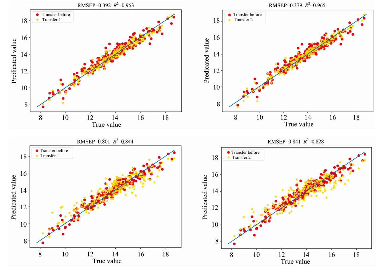 | Fig.7 The prediction results of the transfer of the four models by using 30 samples |
It can be seen from Fig.7 that the model's predicted value which transfers the parameters of the fully connected layer is generally closer to the true value than before the transfer. However, most of the predicted values of the models that re-added fully connected layers for transfer are offset. Some samples are seriously offset and even unpredictable. In order to avoid contingency and to further study the performance of the model after the transfer, the division ratio of the sample was changed, and then the prediction was made. The results are shown in Table 6.
| Table 6 The transfer prediction results of four models with different training set sizes |
Increasing the training sample improves the prediction performance of the transferred model. In about 90 samples, the first and second transfer methods hit the model's bottleneck. Since then, the model's prediction performance has stoped rising and started fluctuating within a certain range. After 110 samples, the second and fourth types of the transfer stabilise, but they are still quite different from the first and second types of transfer. It demonstrates that it is difficult to retrain the fully connected layer well when the spectral data set involved in re-calibration is small.
Advanced pattern recognition technology is promoting the remarkable growth of Chemometrics. In this paper, an advanced deep learning model named MSRCNN and a model transfer method adapted to MSRCNN are proposed to improve the prediction performance of the calibration model on one instrument and across the instrument. The experimental results on the drug and wheat data sets show that:
(1) The improved multi-scale fusion residual convolution network can use convolution kernels of different sizes to obtain the features of the spectrum in different sparseness. Without carefully designed pre-processing and wavelength selection algorithms, it has a stronger prediction ability than ordinary convolutional networks and classic Chemometric algorithms.
(2) The problem of model failure can be solved by using transfer learning to transfer the model established on the master instrument to the slave instrument and needs only a few samples spectra of the slave instrument for recalibration. The model with better predictive performance before the transfer also performs better after transferring.
(3) The model transfer method based on the convolutional neural network combined with transfer learning mainly lies in that the feature weights extracted by convolution and fully connected layer training feature weights are similar between different instruments. Therefore, if the convolution layer and full connection layer are transferred imultaneously, the effect is better than that of the untransformed full connection layer when there are few training samples. And whether to freeze the convolutional layer parameters, there is no obvious difference in this study.
The results of similar studies
| DataSet | Studies | RMSE |
|---|---|---|
| IRRC2002 | [20] | 3.219 5 |
| [21] | 2.7 | |
| [22] | 3.3 | |
| [30] | 3.258 | |
| [D1] | 2.501 | |
| ours | 2.289 | |
| IDRC2016 | [20] | 0.664 |
| ours | 0.379 |
Note: [D1]Li Lingqiao. Research on deep learning modeling method of near-infrared Spectroscopy for drug supervision[D]. Beijing University of Posts & Telecommunications, 2020.
| [1] |
|
| [2] |
|
| [3] |
|
| [4] |
|
| [5] |
|
| [6] |
|
| [7] |
|
| [8] |
|
| [9] |
|
| [10] |
|
| [11] |
|
| [12] |
|
| [13] |
|
| [14] |
|
| [15] |
|
| [16] |
|
| [17] |
|
| [18] |
|
| [19] |
|
| [20] |
|
| [21] |
|
| [22] |
|
| [23] |
|
| [24] |
|
| [25] |
|
| [26] |
|
| [27] |
|
| [28] |
|
| [29] |
|
| [30] |
|
| [31] |
|
| [32] |
|
| [33] |
|