The single fluorescence excitation emission matrix (EEM) is bilinear and can be analyzed by principal component analysis (PCA). The MDR-PCA method firstly deducts the scattered interference data, and then uses the remaining fluorescence data to recover the deducted parts through the defect data reconstruction algorithm during the iterative process of the principal component analysis, completely avoiding the interference of the scattered signal to the fluorescence analysis. The MDR-PCA method can be divided into the following main steps:

(1)The scattering region in the EEM spectral matrix Z is identified. For Rayleigh scattering, it is generally the diagonal region of |EM-EX|≤ 10~15 nm;

(2)Set the weighting matrix W of the same size as Z. The part of scattering data in corresponding matrix Z is set to 0 and the rest is set to 1;

(3)The data of spectral scattering region can be set as defective data, such as 0 or nan;

(4)In the iterative process of principal component analysis (PCA) of EEM matrix Z, the missing data in the matrix is reconstructed using the score vector t and the load vector p calculated in each step;

pT=tT×Z(1)

p=p/|p|(2)

Z=Z×W+t×pT☉(1-W)(3)

t=Z×p(4)

Z=Z☉W+t×pT(1-W)(5)

(5)Iterative calculation to convergence, convergence loss function does not take into account the missing data part;

(6)If you need to calculate more principal components, make Z_k+1=Z_k-t_k× pkT, continue the calculation of step (4)— (5);

(7)Replace the scattering region with the principal component reconstructed defect region to obtain a repaired spectral matrix X:

X=Z☉W+T×pT☉(1-W)(6)

This method not only eliminates the scattering interference, but also makes full use of the effective information in the fluorescence spectrum matrix to repair the scattering region, which is beneficial to the non-destructive analysis of the three-dimensional fluorescence spectrum.

The expression of the trilinear model is:

xijk=∑n=1Nainbjnckn+eijki=1, 2, …, I; j=1, 2, …, J; k=1, 2, …, K(7)

There, x_ijk is an element of the three dimensional data matrix X; e_ijk is a constituent element corresponding to the error matrix E; a_in, b_jn and c_kn are the elements of the matrix A, B and C, respectively.

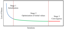
According to the change of loss function

∑i=1I∑j=1J∑k=1Kxijk-∑n=1Nainbjnckn2

the iterative optimization process of trilinear decomposition algorithm is decomposed. The loss function increases with the number of iterations as shown in Figure 1. From the figure we can see that from the beginning of the random initial value of the algorithm to the convergence of the analytical results with physical meaning, this process can be roughly divided into three parts: Initial value optimization process, algorithm optimization process and algorithm convergence process.

Fig.1

	Figure Option ViewDownloadNew Window
	Fig.1 Loss function change process

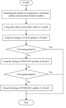
Comparing the performance of the ATLD, SWATLD, and PARAFAC algorithms with the division of the iterative process, it can be seen that the three algorithms are more important than optimizing the different parts of the iterative process. Therefore, we can try to use the above three algorithms in the corresponding part to realize the complementary advantages of each algorithm. The combination of the three algorithms described above is implemented in the following manner: Firstly, the random initial value is optimized by ATLD, then the convergence result of ATLD is further optimized by SWATLD. Finally, the result of SWATLD is optimized by using PARAFAC to realize the trilinear decomposition of data. This algorithm is called the algorithm combination methodolog (ACM).

When the data structure is simple, there is no obvious difference in the results obtained by each algorithm. Therefore, ACM can be further optimized to make it more efficient in data parsing. From the experience of application, the loss function of SWATLD will decrease monotonously until it converges when the data structure is relatively simple. This phenomenon is incorporated into ACM. If the loss function of SWATLD converges monotonously, the result will be further optimized without using PARAFAC. Otherwise, you need to introduce PARAFAC. The whole process of ACM is shown in Fig.2.

Fig.2

	Figure Option ViewDownloadNew Window
	Fig.2 Algorithm combination methodology data analysis flow chart

Hitachi F-7000 fluorescence spectrometer was used for the experiment. Parameter settings: excitation wavelength range 250~430 nm, emission wavelength range 310~520 nm, step length is 5 nm- slit width is 10 nm; scanning speed is 12 000 nm· min^-1, PMT voltage is 400 V. Each sample was measured three times in parallel, and the average value was taken as the fluorescence spectrum of the sample.

Three product oils (0^# diesel, 95^# gasoline, and ordinary kerosene) were selected as representatives of petroleum-based materials, and carbon tetrachloride as solvent. Separately take 1g of each of 0^# diesel, 95^# gasoline, and ordinary

kerosene in a 100 mL volumetric flask with an electronic balance, and add CCl₄ to fully dissolve to obtain a standard solution of 10 000 mg· L^-1 of three oils. Separately take three different standard solutions of different volumes in Eighteen 50 mL volumetric flasks and add CCl₄ to volume to prepare samples of different concentrations. Number them: 1^#— 11^# are calibration samples, and 12^#— 26^# are prediction samples. The concentration of mineral oil in each sample is shown in Table 1.

Table 1

Table 1

Table 1 The concentration of oil in the sample (mg· L-1) Samples 0#Diesel 95#gasoline kerosene Samples 0#Diesel 95#gasoline kerosene 1 100 0 0 14 30 70 0 2 0 100 0 15 20 80 0 3 0 0 100 16 40 28 0 4 80 10 0 17 60 17 0 5 60 20 0 18 80 10 0 6 50 30 0 19 50 40 65 7 70 25 5 20 25 50 50 8 60 10 25 21 60 25 25 9 30 20 50 22 80 10 10 10 10 25 50 23 30 35 13 11 5 50 80 24 50 22 26 12 50 25 0 25 70 14 39 13 75 50 0 26 40 30 20

Table 1 The concentration of oil in the sample (mg· L-1)

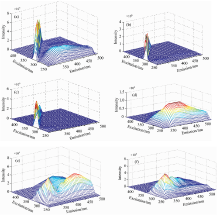
In the excitation-emission fluorescence spectral matrix (EEM) of diesel, gasoline and kerosene carbon tetrachloride solution, Rayleigh scattering occurs in the region where the excitation wavelength is similar to the emission wavelength, as shown in Fig.3(a), (b) and (c). The Rayleigh scattering signal has a high intensity, sometimes up to several orders of magnitude higher than the fluorescence signal, and its intensity is inversely proportional to the fourth power of the wavelength. Because the Rayleigh scattering region does not accord with bilinear and trilinear, it often causes great damage to the results of fluorescence spectrum analysis, so it should be eliminated as far as possible in fluorescence spectrum analysis. Using the MDR-PCA method, the region |EM-EX|≤ 8 nm is set as the data defect area and the scattering region in the EEM spectrum is corrected. The corrected EEM spectrum is shown in Fig.3(d), (e) and (f). Compared with Fig.3(a), (b) and (c), it can be seen that the EEM spectrum has a smooth transition in the scattering region. The MDR-PCA method can effectively utilize the normal fluorescence signal and eliminate the influence of the scattering interference signal.

Fig.3

Figure Option ViewDownloadNew Window

Fig.3 3-D fluoresence spectrum of three standard samples (a): 3-D fluoresence spectrum of 0# diesel without calibration; (b): 3-D fluoresence spectrum of 95# gasoline without calibration; (c): 3-D fluoresence spectrum of kerosene without calibration; (d): 3-D fluoresence spectrum of 0# diesel after eliminating scattering; (e): 3-D fluoresence spectrum of 95# gasoline after eliminating scattering; (f): 3-D fluoresence spectrum of kerosene after eliminating scattering

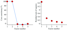
Scanning calibration samples 1#— 6# and prediction samples 12#— 18#, and after data preprocessing to remove the scattering, a 13× 37× 43 three-dimensional matrix X₁ is constructed. Before using the ACM algorithm, it is important to determine the number of factors in the analysis object. In this paper, the factor number of three-dimensional data matrix of experimentally measured is estimated by using core consistancy diagnostics method and residual analysis method^{[13, 14]}. The changes of the core consistancy value and residual sum of squares with the number of factors are shown in Fig.4.

Fig.4

	Figure Option ViewDownloadNew Window
	Fig.4 X1 nuclear consistent diagnosis results and residual square sum analysis results

When the factor number is 1 or 2, the kernel concordance is 100%, and when the factor number is 3, 4, 5, the nuclear concordance coefficient decreases significantly. When the number of factors increases, the sum of squared residuals decreases monotonously, that is, the decomposition error can be reduced by selecting more factors. According to the two indexes, the selected factor number is 2, which is consistent with the actual situation of sample preparation. For the 2-factor analysis, the excitation and emission spectra obtained by the discrimination are shown in Fig.5. It can be seen that the spectrum after the resolution of diesel and gasoline has high spectral similarity and good reproducibility compared with the actual measurement, which qualitatively shows that ACM decomposition has good resolving power for mixed oils.

Fig.5

	Figure Option ViewDownloadNew Window
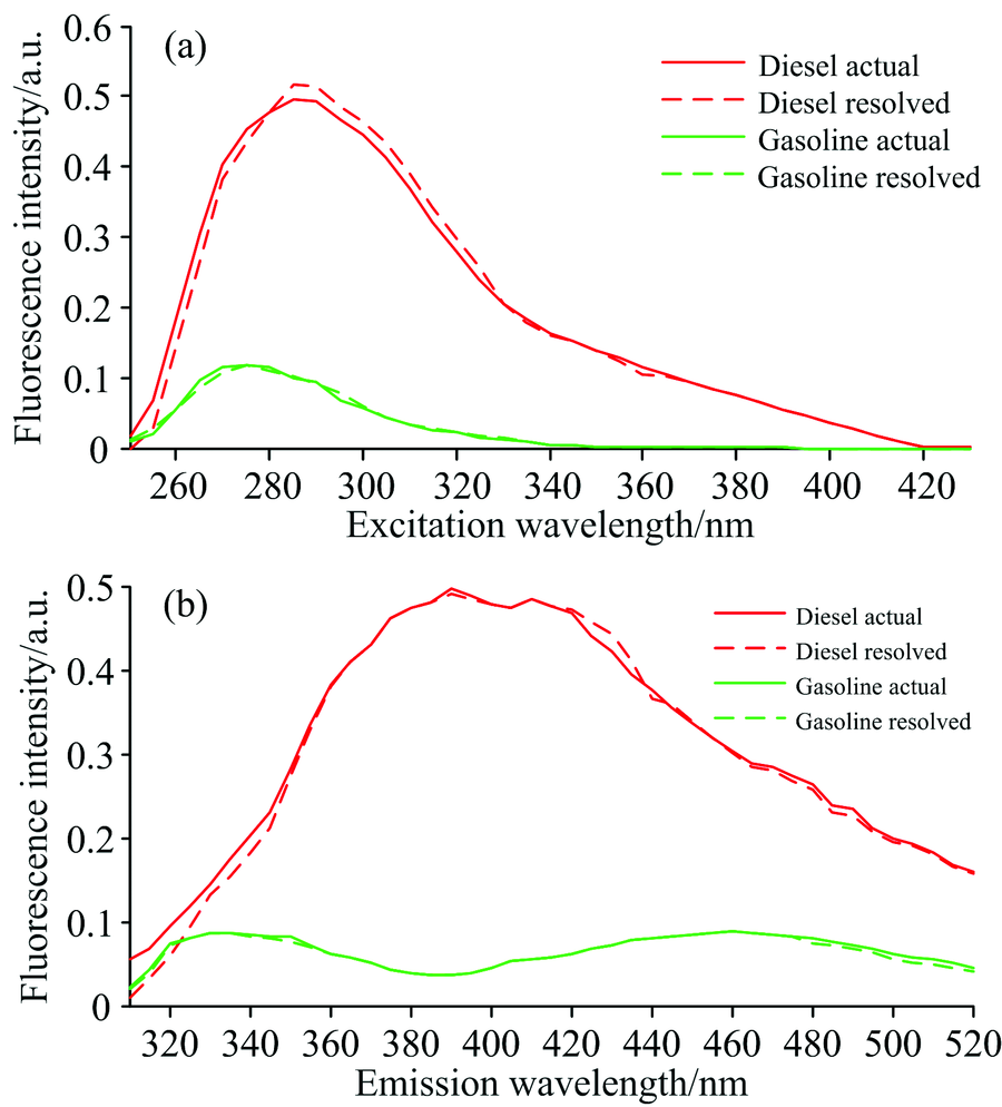	Fig.5 Real spectra and ACM decomposition spectra of diesel and gasoline

The concentration of each oil component in the predicted sample was predicted, and the result was expressed as recovery rate. The expression of the recovery rate is

R=(A/B)×100%(8)

There, A is the predicted concentration; B is the real concentration.

The predicted concentrations of diesel and gasoline in the 12^#— 18^# predicted samples and the sample recovery rate are shown in Table 2. It can be seen from the table that the predicted concentration of diesel and gasoline is very close to the true concentration, the average recovery rate is 97.36% and 97.26% respectively. The quantitative analysis indicates that the ACM decomposition algorithm has a good resolution for diesel and gasoline.

Table 2

Table 2

Table 2 Predicted concentration and recovery of ACM decomposition of diesel and gasoline Samples Predicted concentration/(mg· L-1) Recovery/% Average recovery/% Diesel gasoline Diesel gasoline Diesel gasoline 12 51.82 20.62 103.6 82.5 13 73.90 45.23 98.5 90.5 14 26.33 76.44 87.8 109.2 15 19.66 83.92 98.3 104.9 97.36 97.26 16 38.92 27.63 97.3 98.7 17 58.61 16.77 97.7 98.6 18 78.65 9.64 98.3 96.4

Table 2 Predicted concentration and recovery of ACM decomposition of diesel and gasoline

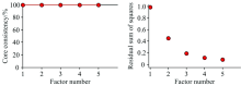
Scanning calibration samples 7^#— 11^# and prediction samples 19^#— 26^#, and after data preprocessing to remove the scattering, a 13× 37× 43 three-dimensional matrix X₂ is constructed. The changes of the core consistancy value and residual sum of squares with the number of factors are shown in Fig.6.

Fig.6

	Figure Option ViewDownloadNew Window
	Fig.6 X2 nuclear consistent diagnosis results and residual square sum analysis results

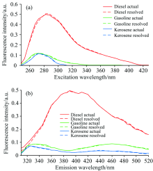
Assuming that there are five factors, the degree of core consistency is always close to 100%, that is, from the point of view of core consistency, it is acceptable to use one to five factors for ACM analysis. Analysis of the sum of squared residuals found that the sum of the squared residuals of the 3-factor analysis was significantly lower than that of the 2-factor analysis, but it was less different from the sum of the squared residuals of the 4-factor analysis. The known samples are made up of three substances: diesel, gasoline and kerosene. If the ACM analysis of F=3 is used according to the actual condition of sample preparation, the excitation and emission spectra can be resolved as shown in Fig.7. It can be seen that the resolving spectra of diesel, gasoline, and kerosene have higher similarity with the actual spectrum and good repeatability, which qualitatively shows that ACM decomposition has good resolution of oil mixtures.

Fig.7

	Figure Option ViewDownloadNew Window
	Fig.7 Real spectra and ACM decomposition spectra of diesel, gasoline, and kerosene

Table 3 lists the predicted concentrations and sample recoveries of diesel, gasoline and kerosene from ACM decomposition in the predicted sample of 19^#— 26^#. The average recovery rates of diesel, gasoline, and kerosene were 97.08%, 97.34%, and 97.25% respectively. The fitting accuracy is high and the concentration prediction deviation is small. It can be seen that ACM decomposition algorithm also has good resolution ability for three or more kinds of mixed oil.

Table 3

Table 3

Table 3 Predicted concentration and recovery of ACM decomposition of diesel, gasoline and kerosene Samples Predicted concentration/(mg· L-1) Recovery/% Average recovery/% Diesel gasoline kerosene Diesel gasoline kerosene Diesel gasoline kerosene 19 47.81 38.68 64.30 95.6 96.7 98.92 97.08 97.34 97.25 20 23.64 48.94 47.83 94.6 97.9 95.66 21 59.05 24.51 24.02 98.4 98.0 96.08 22 79.92 9.62 9.75 98.7 96.2 97.5 23 28.98 33.90 12.73 96.6 96.9 97.9 24 48.77 21.68 25.54 97.5 98.5 98.2 25 68.67 13.73 37.54 98.1 98.1 96.3 26 38.85 28.91 19.47 97.1 96.4 97.4

Table 3 Predicted concentration and recovery of ACM decomposition of diesel, gasoline and kerosene