


中高层OH自由基在紫外波段的临边散射辐射正演模拟与敏感性分析
[方雪静1, 2, 3  , 熊伟
, 熊伟1, 3, * , 施海亮1, 3 , 罗海燕1, 3 , 陈迪虎1, 3 ]
, 熊伟|
|


OH自由基是中高层大气中重要的氧化剂, 决定着臭氧以及其他温室气体的浓度变化, 甚至气候变化。 为了实现中高层大气OH自由基的精细探测与精确反演, 需要构造正演模型, 模拟得到仪器接收到的大气中的 A2 Σ+- X2 Π(0,0) 309 nm波段的太阳共振荧光发射信号。 本文基于分子光谱能级跃迁理论计算得到OH(0,0)振动能级上的荧光发射率因子 g, 结合辐射传输模型SCIATRAN模拟出的太阳辐照度和观测视线路径上的OH柱量, 模拟出OH荧光发射光谱, 叠加上大气背景光谱并卷积仪器函数, 最终模拟得到仪器接收的包含OH浓度信息的光谱。 模拟结果与国外在轨仪器MAHRSI(Middle Atmosphere High-Resolution Spectrograph Investigation), SHIMMER(Spatial Heterodyne Imager for Mesospheric Radicals)的在轨实测结果一致性较好。 还分析了影响模拟结果的因素, 在之后的正演过程中加以修正, 使正演模型更接近实际辐射传输过程。
Biography: FANG Xue-jing, (1991—), female, PhD, Anhui Institute of Optics and Fine Mechanics, Hefei Institutes of Physical Science, CAS,e-mail: fxj126@mail.ustc.edu.cn
Hydroxyl, one of the principal oxidants in the atmosphere, determines the density of ozone and other greenhouse gases even the change of climate. In order to achieve high resolution vertical profiles of OH radical in mesosphere, an accurate forward model should be built up for its retrieval. In this paper,this forward model simulates limb-scattered signal including OH solar resonance fluorescence around 309 nm. We calculate OH band rotationalemission rate factor g based on molecular spectroscopy theory, and combine it with OH slant column calculated by SCIATRAN to synthesize OH fluorescence emission spectra. By superimposing atmospheric background signal and do a convolution with instrument line shape function, we could obtain a simulated spectra containing OH concentration information.These results are in good agreement with previous measurements by MAHRSI (Middle Atmosphere High-Resolution Spectrograph Investigation) and SHIMMER (Spatial Heterodyne Imager for Mesospheric Radicals). Then we analyze several factors that may influence the forward model. By modifying these parameters, forward model could be more accurate and closer to the actual radiative transfer process in the future.
The hydroxyl(OH) radical is the most important oxidizing agent in the middle atmosphere, though its mixing ratios are only parts per trillion or billion by volume[1]. OH chemistry dominates ozone destruction above about 40 km and also serves as a proxy for upper mesospheric water vapor[2]. Knowing about OH radical will help to understand the atmospheric components and photochemistry events in mesosphere.
Measurements of mesospheric OH have been performed from aircraft, balloons, and satellites[3, 4]. In mid-1990s, Middle Atmosphere High-Resolution Spectrograph Investigation (MAHRSI)[1] obtained the first global map of OH in mesosphere. In 2007, Spatial Heterodyne Imager for Mesospheric Radicals (SHIMMER)[5] measured the solar resonance fluorescence of OH over the diurnal cycle[3]. It was an instrument that used Spatial Heterodyne Spectroscopy (SHS) technique. Its measurement had a better agreement with standard photochemistry model than that of MAHRSI.
Forward model for MAHRSI was worked out by the basic radiative transfer equation. It considered OH fluorescence, absorption by ozone, Rayleigh scattering by N2 and O2 as well as self-absorption. The atmosphere is modeled as a series of concentric shells of thickness 2 km. The species density is assumed to be constant within each spherical shell. SHIMMER’ s forward model for OH is similarly the same when being used for the MAHRSI retrievals.
Retrieval is a process to get useful information from measurements. While forward model is the foundation of retrieval. In order to retrieve OH vertical profiles from limb measurements, an accurate and effective forward model is needed. Our work combines basic idea of MAHRSI’ s forward
model and convenient radiative transfer model software to make a higher vertical resolution simulation of limb-scattered radiation. In addition, by making use of relatively large electronic cross section of OH around 309 nm[6], we could work out its fluorescence spectra which is excited by solar energy. This fluorescence signal will be detected together with background signals in limb mode. We will get OH details by analyzing this limb-scattered radiation signal.
Forward model describes the process that the radiation transfers from the source to the receiver.
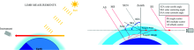
The sun is the source in passive remote sensing. As is shown in Figure 2, the solar energy transfers through the atmosphere to the ground, the detector on the track receives limb-scattered signal including information of ingredients in atmosphere, such as trace gases, aerosols and the land surface. In this mode, the line of sight has a long distance and it is more sensitive to trace gas vertical distribution. The price of high vertical resolution is relatively bad horizontal resolution[7].
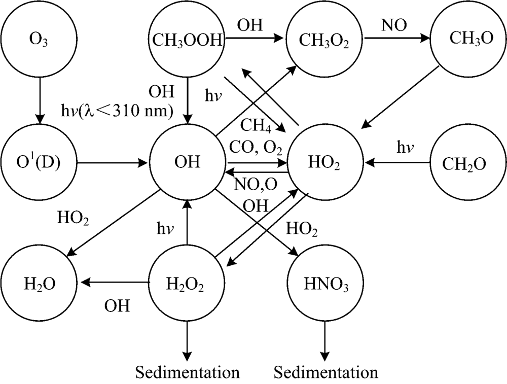 | Fig.1 Main OH photochemistry actions in atmosphere |
 | Fig.2 Limb mode geometry |
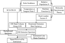
We have built up a modified forward model as is shown is Figure 3, in this forward model, there are three basic components: rotational emission rate factors g, OH slant column along LOS and atmospheric background signal. By synthesizing them together we could obtain a simulated spectrum received by the instrument and OH radiance profiles. The instrument here is a detector used SHS technique which is similar to SHIMMER.
 | Fig.3 Forward model structure |
SCIATRAN[8] covers the spectral range 175.44 nm~4 000 μ m comprising the eight spectral channels of the SCIAMACHY (Scanning Imaging Absorption spectroMeter for Atmospheric CHartographY) instrument. SCIATRAN has been developed to perform radiative transfer modeling in any observation geometry appropriate to measurements of the scattered solar radiation in the Earth’ s atmosphere.
SCIATRAN can build up atmospheric models including 23 kinds of trace gases, Rayleigh scattering, aerosols and clouds. It has stable input parameters and sufficient databases including aerosols, surface reflectance models and suitable ILS (Instrument Line Shape). Above all, it runs quite fast in the retrieval module[8, 9, 10]. The latest version of SCIATRAN is 3.8.13, and we use version 3.3.2.
We complement SCIATRAN’ s databases to meet our needs, including adding high-resolution NSO (National Solar Observatory) solar spectrum and OH line parameters in ultraviolet band from ‘ HITRAN on the web’ databases.
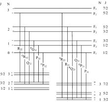
OH radical’ s solar resonance fluorescence is the excited emergent light by solar radiation around 309 nm. A2Σ + is the excited state and X2Π is the ground state in A2Σ +-X2Π (0, 0) transition. Due to Hund’ s cases (a) and (b) and Λ doubling of X2Π [11], these two levels split. Following selection rules for this transition, some rotational transitions are allowed in Figure 4[12].
 | Fig.4 A2Σ +-X2Π (0, 0) allowed transitions |
Rotational emission rate factor g measures the emission efficiency of a molecule, which means when being excited by solar radiation, how many photons can emit per second per molecule. Suppose that in mesosphere with thin optical depth, the observed intensity 4π Iv'v″ can be related to the g factor[13],
where η (z) is the column abundance along the viewing path and can be calculated by SCIATRAN. The g factor is a function of temperature T and tangent altitude z.
Rotational emission rate factor g may be calculated by the expression,
Where the values of following parameters are the same as that in Stevens and Conway’ s paper.is the vibrational band branching ratio and fv'0 is the band oscillator strength. S is Hö nl-London factors, The branching ratiois ω 00=A00/Σ A0v″ taken to be 1.00. The constant
There are other parameters need to be calculated using molecular spectroscopy theory, HITRAN databases[14], energy level information J', J″ and low energy E0. NJ(T) is the relative population in rotational level J at temperature T. It could be calculated by Boltzmann distribution.
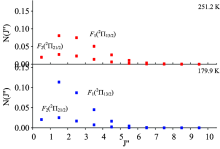
If the hydroxyl molecules in the atmosphere are in thermal equilibrium, the rotational population distribution can be described by the Maxwell-Boltzmann distribution law[6, 15, 16].
where h is Plank’ s constant, c is the speed of light, E(J) (cm-1) is the energy of the X2Π state, k is the Boltzmann constant, T is the equilibrium temperature in K, and Q(T) is the partition function. The partition function Q(T)=QvQr, where the vibrationalpartition function Qv is
ω e is the first order vibrational constant which is equal to 3 737.761 cm-1. Because of this large energy separation between vibrational levels, Qv≈ 1 at middle atmospheric temperatures.
The rotational partition function Qr is
Thus, NJ(T) is worked out as is showed in Figure 5.
 | Fig.5 Calculated relative population of the ground rotational states of OH |
Solar irradiance showed in Figure 6 with a high spectral resolution of 3.5× 10⁻⁴ nm in this band (308.2~309.8 nm) used in this calculation is from NSO (National Solar Observatory)[17] and it has already been modified so that it’ s the direct irradiance at the observation point.
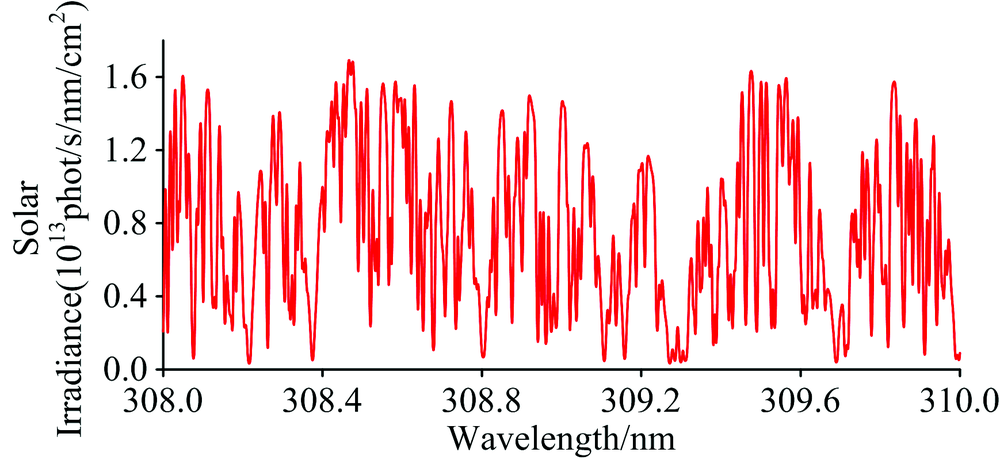 | Fig.6 Solar irradiance used in calculation of g factors |
The g factors results compared with Stevens and Conway’ s work is shown in Figure 7. We choose the temperature 200K because the previous works have published a result at this temperature which is nearly the temperature at 70 km in mesosphere. We can tell that our results are about 60% larger because of the larger solar irradiance. And change of HITRAN databases of OH molecule in these years may cause different relative intensity.
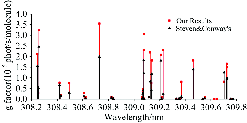 | Fig.7 g factors calculation comparison with previous work at 200 K |
We use the profiles of OH, O3 and other trace gases in SCIATRAN B2D profiles databases to match the forward model algorithm of SCIATRAN. In forward model simulation, we calculate 45 km to 85 km in 1 km step.
Slant column is the column abundance along the viewing path, which could be calculated by the absorption of OH along the LOS. Thus the final signal may include the OH abundance information which can be retrieved from formula (1).
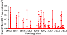
The limb mode has a long viewing path which leads to a relatively large slant column. Under optically thin condition, the emission energy may transfer from the observation point to the instrument without attenuation. The slant column in 70 km tangent point calculated by SCIATRAN with parameter settings listed in Table 1 is showed in Figure 8. Each wavelength has different value because the algorithm used in slant column calculation depends on the absorption characteristics of OH. This may mean that stronger absorption line corresponds to relatively larger slant column and the integration over the band should be equalthe to column abundance in unit molecules· cm-2. The spectral band we choose is 308.2~309.8 nm which meets the need of our spatial heterodyne spectrometer that intends to detect mesospheric OH radicals. At the same time, we calculate solar direct radiance at each tangent point.
| Table 1 Main input parameters settings in SCIATRAN |
 | Fig.8 Calculated slant column at 70 km for each wavelength |
Figure 9 shows simulated background spectrum in 70 km with the same settings in slant column calculation. The shape is almost like the solar irradiance because it consists of Rayleigh scattering, extinction of OH itself, aerosols and other trace gases without OH emissions, whose value depends on atmospheric condition including solar irradiance, aerosol, cloud, trace gases, surface and observation geometry. In this case, we don’ t consider cloud due to its ignorable disturbance in mesospheric limb mode.
 | Fig.9 Calculated background signal |
We add the product of g factors and slant column to the background signal, then do a convolution with the instrument line shape function which is a Gaussian function with a FWHM of 0.015 nm. This FWHM value corresponds to the spectral resolution of our spatial heterodyne spectrometer.
Using this forward model, we also simulate OH emission signals at different altitudes between 45 and 85 km. The OH intensity increases as the height goes down, but combining Figure 10 and Figure 11, we can tell that at 40 km, OH signal is difficult to be distinguished from the total signal because of rapid increasing of Rayleigh scattering signal in lower altitudes.
 | Fig.10 Simulated results at 45 and 70 km. In upper two panels are the synthetic signal, background signal and the OH emission signal at 70 km. In lower two panels are ones at a different tangent height of 45 km |
 | Fig.11 OH emission intensity in different tangent height |
Figure 12 shows OH density and radiance profiles between 60 and 85 km. We choose this altitude range for analyzing because our forward model is more applicable and accurate in this area and previous research such as SHIMMER has a reliable result only in this range. From this result we can tell that the intensity of OH emission signal is related to the density at different tangent heights. The shape of the OH radiance profile is similar to that of density profile.
 | Fig.12 Input OH density profile and simulated OH radiance |
 | Fig.13 Observation radiance with different solar zenith angles and azimuth angles |
There are some important parameters in forward model which would have an effect on the results, which would even influence the retrieval accuracy. Geometric parameters, aerosols and OH concentration are considered in this sensitivity analysis. Default settings are listed as in Table 1.
In the mesosphere, land surface parameters are relatively small, so the most important factors in limb observation mode is the geometry parameters including solar zenith angle, solar azimuth angle and tangent point position. These three parameters determine the position of the observation point.
The parameter of “ Azimuth angles” here defines the values of the relative azimuth angles of line-of-sight with respect to the sun. The value of 0° means instrument is pointed into the solar direction. The intensity decreases rapidly with increasing SZA near 90° because in this position, the observation geometry is going into twilight mode like in Figure 14(b). In azimuth angles sensitivity analysis, when SAA=180° , the sun and the instrument are in a line by two sides, so more transmitted and scattered solar radiation are transferred into the instrument.
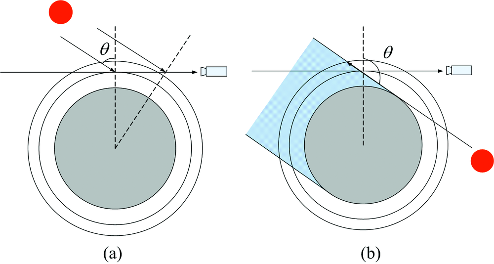 | Fig.14 Geometry in (a) nontwilight (b) twilight |
The sum of the aerosol scattering coefficient and the aerosol absorption coefficient yields the aerosol extinction coefficient for each aerosol type. These three coefficients have the unit of an inverse length (km-1).
We use user-define aerosol settings and set AOT in range of 0 to 5 by the step of 0.05 with reference wavelength of 308 nm. For mesospheric aerosol, scattering coefficient is much larger than absorption coefficient[6]. Therefore, larger AOT brings out larger limb-scattered radiation. Figure 15 proved this statement.
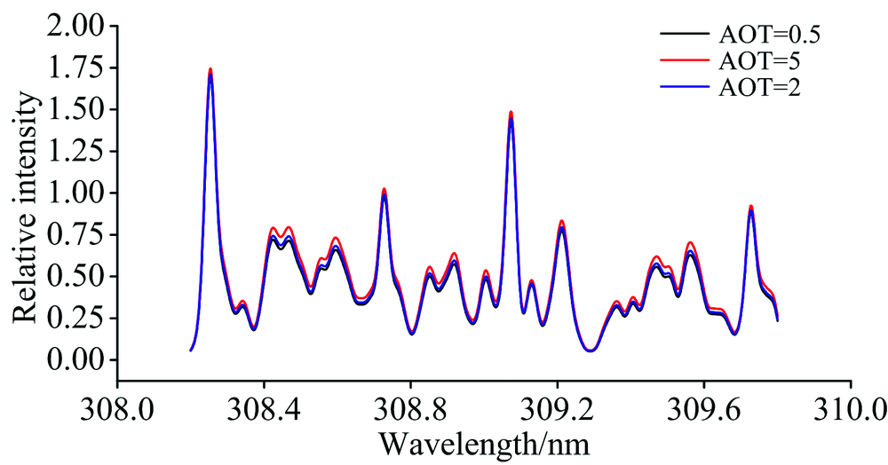 | Fig.15 Limb-scattered radiance at 70 km with different AOT |
We do a 10% perturbation to OH concentration by step of 1 km and simulate limb-scattered radiance in 41 tangent heights between 44 to 84 km.
The relationship between limb-scattered radiance and OH concentration could be described by a parameter called “ Weighting Functions” . It’ s a matrix usually used in retrieval, whose element could be expressed as
Where Ij is the limb-scattered radiance and nk is the OH concentration in the tangent height j, Δ is the difference before and after perturbation.
From Figure 16, we can tell the sensitive tangent height range for OH is above 70 km. That is to say, it’ s more effective and would have higher accuracy of OH’ s retrieval in this height. The weighting function has different maximum intensity in different wavelength due to relative intensity of OH emission line.
 | Fig.16 OH Weighting functions in different wavelength |
(1) Factors in g factor calculation
Formula (1) is applicable under optically thin conditions and in absence of quenching. If atmospheric optical thickness could not be neglected, the results using this formula may not be accurate. That is to say, the effective range for this algorithm is at least 50 km above. The higher the altitude is, the more accurate the forward model is. In lower altitude, the air is becoming thicker, more N2 and O2 may influence the stability of OH excited state. In another way, the background signal may become too large to distinguish OH signal from it.
We can see that in formula (2) there are so many parameters in calculating g factor. Solar irradiance and temperature are the two most important factors in this calculation, which need to be as accurate as possible for this model.
(2) Factors in SCIATRAN simulation
There are common errors in forward model which are the differences between the input conditions and the actual conditions.The analysis should be discussed by combining measurements and retrieval results. In this case, we definitely should build forward model as close as to the actual situation to reduce the retrieval uncertainty and errors.
(3) Sensitivity analysis
In limb mode in mesosphere, features of land surface wouldn’ t matter a lot for scattered signal. And thinner optical condition may lead to less extinction of intensity. Measurement of OH in mesosphere is seemed to be influenced by the OH concentration itself and long viewing path. OH density profile peaks at about 70 km and the background signal is rather small, so it’ s easier to separate OH signal from Rayleigh scattered signal. Accuracy of forward model and retrieval depend on these atmospheric parameter settings definitely. We would make a detailed analysis in future works which focus on clouds or other trace gases such as ozone.
We calculate OH band rotational emission rate factors g based on molecular spectroscopy theory. What’ s more, combining with solar irradiance and slant column calculated by SCIATRAN, we obtain the simulated received signals by the spatial heterodyne spectrometer at 50~80 km. This spectrum contains OH concentration information along the viewing path. By using an effective retrieval algorithm, OH density at each altitude could be worked out using this forward model. Sensitivity analysis of several atmospheric parameters is also done to give a brief understanding of components which have effects in radiative transfer model. It is important to build an accurate forward model, especially for OH radicals in the order of magnitude of ppbv. This forward model provides a foundation for retrieving atmospheric OH radical in high precision and also much valuable information for researching on the mesospheric photochemical processes.
The authors of this study would like to thank Key Laboratory of Optical Calibration and Characterization of Chinese Academy of Sciences for funding this research. We wouldlike to thank Dr. Alex Rozanov from Institute of Environmental Physics/Institute of Remote Sensing, University of Bremen, Germany for helpful advices in using SCIATRAN.
The authors have declared that no competing interests exist.
| [1] |
|
| [2] |
|
| [3] |
|
| [4] |
|
| [5] |
|
| [6] |
|
| [7] |
|
| [8] |
|
| [9] |
|
| [10] |
|
| [11] |
|
| [12] |
|
| [13] |
|
| [14] |
|
| [15] |
|
| [16] |
|
| [17] |
|