

基于集群方法(ER)的近红外光谱转移集优化法
[郑开逸1  , 张文
, 张文1 , 丁福源1 , 周晨光1 , 石吉勇1 , 丸仲良典2 , 邹小波1, * ]
, 张文]
|
|


近红外光谱因为具有小成本、 易操作、 低耗时等优点, 所以广泛用于食品领域。 作为一种间接的检测方法, 近红外光谱检测需要建立光谱和浓度之间的统计模型。 但是, 一种条件下建立的模型在另一种检测条件下会失效。 针对此问题, 重新建模可以加以解决, 但是重新建立光谱与浓度之间的模型非常繁琐耗时。 此时, 模型转移可以在避免重新建模的情况下, 通过光谱校正, 保证预测精度。 在模型转移中, 已经建立好模型的光谱称为主光谱( A), 不用建立模型, 而只用主光谱模型预测的光谱称为从光谱 ( B)。 模型转移方法的步骤是, 先在校正集中选择一些样本作为主光谱的转移集( At), 然后选择从光谱中浓度和 At相同的光谱, 以此作为从光谱的转移集( Bt)。 通过 At和 Bt构建模型转移矩阵。 最后将需要校正的从光谱( Bv)乘以上述的转移矩阵中, 即可获得校正后的从光谱( Bnew)。 此时, Bnew就可以用主光谱的模型来直接预测。 在模型转移中, 转移集样本的选择对模型校正至关重要。 目前, 转移集的样本通常从光谱之间的距离而非模型转移误差获得。 但是, 转移误差对模型转移结果的验证至关重要, 故该研究出了基于集群分析的集群优化法(ER)并将其用于优化KS方法产生的转移集样本。 ER先用随机方法建立转移集的多个子集合, 并计算每个子集合的转移误差。 然后, 对某一个样本, 计算包含这个样本的子集合转移误差均值。 最后, 选择转移误差均值较低的样本作为新转移集样本进行模型转移。 以玉米数据测试了ER算法。 结果显示, 对于典型相关分析-有信息成分提取法(CCA-ICE)、 直接校正法(DS)、 分段直接校正法(PDS)、 光谱空间转化法(SST)这些常见的模型转移方法, 相比于KS样本选择方法, ER方法可以找出重要的转移集样本, 进而显著降低模型转移误差。
, ZHANG Wen
Biography: ZHENG Kai-yi, (1983—), associate researcher, School of Food and Biological Engineering, Jiangsu University e-mail: kaiyizhengjsu@126.com
The near-infrared spectra has been widely used in the food region with advantages of low measurement cost, easy operation, and fast analysis rate. An indirect analytical method should calibrate a feasible model between spectra and concentrations. However, the model calibrated under a specific condition may be invalid for the spectra measured under another condition. Recalibration is a solution to this problem. However, recalibrating the model between spectra and concentration cost much time and workforce. Thus, calibration transfer can correct the spectral deviation to keep the precision of prediction and avoid the expense of recalibration. In calibration transfer, the spectra used for calibrating model are called primary spectra ( A), while those not calibrate model but only use the model of primary spectra are called secondary spectra ( B). The procedure of calibration transfer is selecting samples as transfer set of primary spectra ( At) from the calibration set, while choosing the samples of secondary spectra as transfer-set of secondary spectra ( Bt) who share the same concentrations of At. Then the transfer matrix can be constructed through At and Bt. After that, the corrected secondary spectra ( Bnew) can be obtained by validating a set of secondary spectra ( Bv) multiplying the transfer matrix. Finally, the Bnew can be substituted for the primary spectra model for prediction. In calibration transfer, generating a transfer set is an important procedure. Selecting samples of transfer set is commonly based on the distances of spectra rather than validation errors. However, the transfer errors are important to estimate the power of calibration transfer. Hence, in this paper, ensemble refinement (ER) based on model population analysis has been proposed to refine further the transfer set generated by the KS method. Initially, the ER generates several subsets of a transfer set and then computes the validation errors of each subset. Subsequently the average error of subsets that includes the sample can be obtained for each sample. Finally, the samples with low average errors can be selected as a transfer set for calibration transfer. The corn dataset is used to examine this method. The results exhibited that in calibration transfer methods such as canonical correlation analysis combined with informative components extraction (CCA-ICE), direct standardization (DS), piecewise direct standardization (PDS) and spectral space transformation (SST), ER can select key samples for calibration transfer to reduce the errors, compared with KS method significantly.
Near-infrared spectroscopy (NIR) has been widely used in environmental[1], petrolic[2] and agricultural[3] areas, because of its advantages such as ease of operation, low measurement cost, and fast analysis rate. However, as an indirect analytical method, a feasible model for near-infrared spectroscopy must be developed in advance. Generally, the model calibrated under a specific condition cannot be applied to the spectra under different conditions. Thus, recalibrating a new model is necessary to solve this problem. However, recalibrating the model can be uneconomical and labor-intensive. Thus, calibration transfer can be the solution to this problem.
In the spectra batch of calibration transfer, the samples applied to constructing models are called primary spectra, while the samples which are not calibrated but only use the model of the primary spectra are called secondary spectra[4, 5].
In recent years, several calibration transfer methods have been proposed, including the direct standardization (DS)[6], piecewise direct standardization (PDS)[7, 8], canonical correlation analysis (CCA)[9, 10], spectral space transformation (SST)[11], and so on. Among these methods, CCA-ICE has exhibited promising results for calibration transfer. In addition to calibration transfer models, sample selection methods for transfer sets are also crucial, such as the Kennard-Stone (KS) method[12].
However, the transfer set can only be selected by the distance of samples in the calibration set. Supposedly, refining the transfer set generated by the KS method can further reduce the prediction errors. Meanwhile, less informative samples exist in the calibration transfer which can enlarge the prediction errors. Thus, the samples in the transfer set must be refined further. In recent years, the model population analysis (MPA) being utilized in chemical and/or biochemical data analysis, such as for sample selection methods in multivariate calibration. Similar to multivariate calibration, the transfer set generation in calibration transfer is also a sample selection procedure. Thus, in this study, a transfer set refinement method referred to as ensemble refinement (ER) is proposed, which uses the ideology of MPA to optimize the samples in a transfer set.
The primary and secondary spectra are symbolized as matrices A and B, respectively. The transfer and calibration sets of spectra A are assigned as At and Ac, respectively, while the transfer, validation and prediction sets of spectra B are designated as Bt, Bv and Bp, respectively. The y symbolizes the sample concentrations. At can be obtained from Ac using the sample selection method. Meanwhile, the samples of spectra B with similar concentrations as that At are assigned as Bt.
Similar to the procedure of MPA[13, 14, 15], the ER algorithm includes the following three sections: (1) subset sampling for the transfer set, (2) sub-model building through calibration transfer methods, and (3) random analysis of the root mean square errors of validation (RMSEV) of the generated subsets. The detailed procedure can be shown as follows:
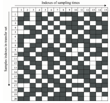
Consider a matrix At for m samples with each row as a sample. Two parameters including ratios of the selected sample to the whole sample (r) and the number of selecting times (N) must be focused on. The samples must be randomly selected from At to generate the subset. After N times of repeatedly sampling, N subsets of the transfer set can be obtained. This procedure is illustrated in Fig.1 where m=20, r=0.6 and N=15.
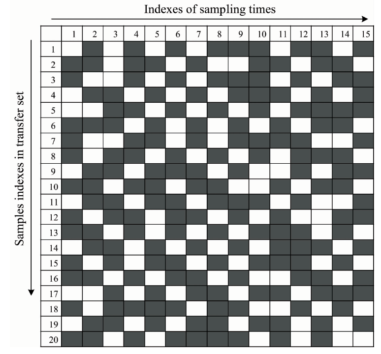 | Fig.1 Illustrative example of the subset sampling in a transfer set The black squares are the selected ones while the white ones not |
Figure 1 shows that the first subset including the 12 samples can be selected among the 20 samples (20× 0.6). Further, other 12 samples can be chosen from another sampling index. Thus, after 15 samplings, 15 subsets of the transfer set can be generated. In Fig.1, the probability of each sample is 0.6, which is identical to the value of r. Furthermore, during the sampling, the selected ratio of a sample is r. Thus, after N samplings, the theoretical number of (Nt) of the sample to be selected can be computed as follows
The insignificant Nt of cannot extract the sample information in a transfer set, while the substantial value of Nt can increase the computation burden. Thus, an optimal Nt value must be fixed. In this study, Nt is set to 100, which implies the theoretical sampling time of each sample is 100. Thus, the former two parameters can be reduced into a single parameter r. With the value of r, the value of N can be computed as follows
Calibration transfer can be generated for each randomly generated sub-dataset to estimate RMSEV (RMSEV1). E.g. in Fig.1, 15 RMSEV1 values can be obtained after 15 sampling times.
After randomly sampling, each sample subset of the transfer set can be applied to the calibration transfer. Thus, the corresponding RMSEV1 values can be obtained after several sampling times. The subsets with RMSEV1 values including the corresponding sample can be obtained for one sample. After that, the average RMSEV1 (mRMSEV1) can be fixed as the subsets with the sample. For example, in Figure. 1, after 15 samplings, the 2nd, 4th , 6th, 8th, 9th, 10th, 12th, 13th and 15th subsets contain the first sample, and thus mRMSEV1 of these samples can be obtained to evaluate the transfer power of the first sample. Similarly, mRMSEV1 of the 1st, 2nd, 4th, 5th, 7th, 10th, 11th, 13th and 14th subsets can be set as the transfer power of the second sample. Based on this, mRMSEV1 of each sample can be obtained.
Evidently, after sampling, the samples with low mRMSEV1 values can be considered candidates for reducing calibration transfer errors. Thus, the samples can be sorted according to their mRMSEV1 values ascending order, and the samples with low mRMSEV1 values can be chosen for calibration transfer. The detailed procedure of the proposed method is given as follows:
In Fig.2, the proposed method includes the following four steps: (1) randomly sampling, (2) obtaining RMSEV1 of each subset, (3) obtaining mRMSEV1 of each sample, and (4) selecting the samples with low mRMSEV1 values. In the proposed method, r and the number of samples in the original transfer set (m) must be adjusted in advance.
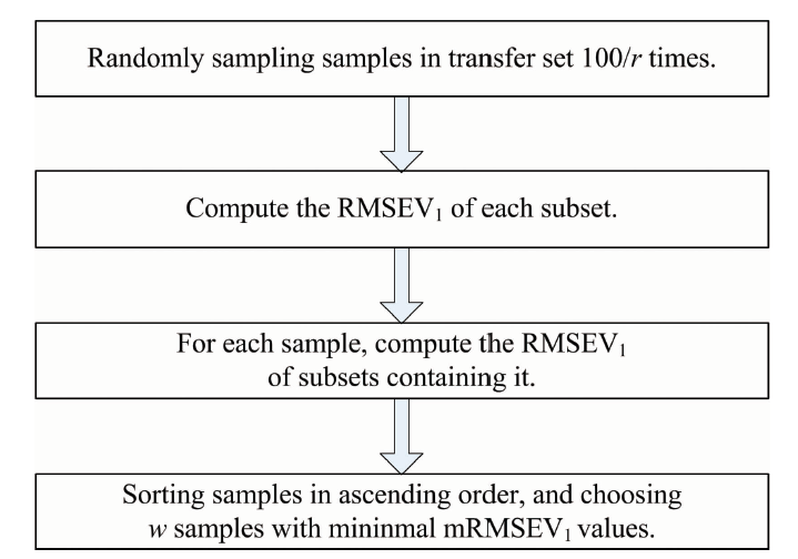 | Fig.2 The procedure of the ER method |
The spectra of the corn dataset scanned on three NIR spectrometers are downloaded from http://www.eigenvector.com/data/Corn/index.html. Each of the three NIR spectra batches includes 80 samples ranging from 1100 nm to 2498 nm. In the three datasets, mp6 and m5 are assigned as primary and secondary spectra, respectively. Meanwhile, the moisture values are set as y.
For primary spectra with 80 samples, after sorting the values of y, the first sample in each of the four contiguous samples (20 samples) is set aside. Thus, the remaining 60 primary spectra samples are considered the calibration set of primary spectra. Moreover, among 60 samples of calibration set of primary spectra, certain samples are chosen as the transfer sets of primary spectra using the KS method. After generating the transfer set of primary spectra, the samples of the calibration set in secondary spectra with similar y values are assigned as the transfer set of secondary spectra.
Moreover, for 20 samples of primary spectra set aside, the samples of secondary spectra with similar y values as that of the former can be retained. Among 20 samples of secondary spectra, the first and second ones of each two contiguous samples are set as prediction and validation sets, respectively.
For the corn dataset, the number of latent variables is optimized as nine. Additionally, the parameters of m and r must be investigated. Because the sampling subset cannot execute CCA-ICE under the condition of m× r< l, the corresponding RMSEV cannot be generated. Thus, the combinations with m× r≥ l must be adopted under different parameter combinations. The results are illustrated below:
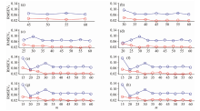
Figure 3, shows that at different combinations of m and r, the RMSEV2 values of the proposed method are nearly lower than those obtained by the KS method. This indicates that the transfer set generated by the KS method can be further refined by using the proposed ER method. In each plot of (c), (d), (e), (f), (g), (h) and (i), with ascending m, RMSEV2 displays a decreasing trend at m< 30. This is because many samples obtained by the KS method facilitate the refinement of ER. Furthermore, after the value of m exceeds 30, RMSEV2 remains nearly constant. Since selecting many transfer samples may generate redundant information for the calibration transfer, m is set to 30.
 | Fig.3 The RMSEV2 of corn dataset at r from 0.2 to 0.9 (plots a to h) and m from 20 to 60 In each plot, the blue and red lines represent RMSEV2 of the KS method and the proposed method, respectively |
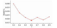
In addition to m, r must be investigated. RMSEV2 at different r values are listed in Fig.4.
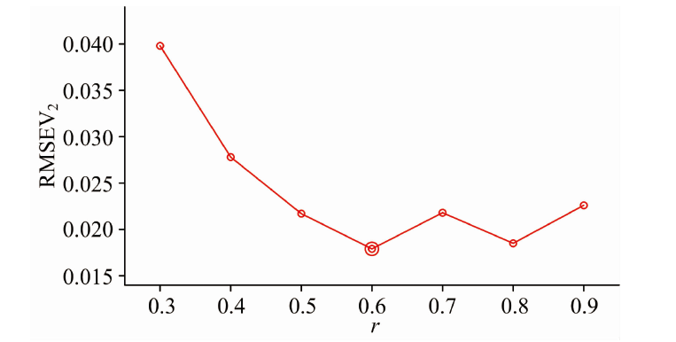 | Fig.4 RMSEV2 of the corn dataset at r ranging from 0.3 to 0.9 at m=30 |
In Fig.4, RMSEV2 achieves the minimal at r=0.6. Thus, r is set to 0.6. After fixing m and r, the variation in RMSEV2 during different w can be examined. The results are displayed below.
Fig.5 indicates that with the increase in w, RMSEV2 decreases at first and achieves the minimum at w=28. At last, RMSEV2 was obtained to be 0.094 2, which is the same as the results without further refinement. Thus, the subset with 28 samples and minimal RMSEV2 can be set as the optimal subset. Fixing the parameters using the validation set, RMSEP of the prediction set must be applied to examine the effect of ER. The results are displayed as follows:
 | Fig.5 Variation in RMSEV2 for subsets with w from 9 to 30 at m=30 and r=0.6 |
In Table 1, it is evident that the ER method can refine the transfer set of CCA-ICE with low RMSEV2 and achieve low RMSEP compared to the KS method. Meanwhile, the commonly used methods such as DS, PDS and SST can also be applied in the ER method. The results are listed in Table 1. In Table 1, DS, PDS and SST utilize ER to refine the transfer set with lower RMSEV2 and RMSEP than the KS method.
| Table 1 Computation errors of corn dataset by KS and ER methods |
Moreover, to further analyze the power of ER, the random sampling method can be used for testing. In each calibration transfer method including CCA-ICE, DS, PDS and SST, the randomly sampling method is used 100 times. In each loop, the calibration, validation and prediction sets are randomly fragmented into the sizes of 60, 10 and 10, respectively. Then, the original transfer sets are generated from the calibration set through the KS method. Subsequently, the samples in the transfer set are further refined by the ER method, and RMSEV2 of the validation set is used to determine the number of samples to be retained. Finally, the refined and non-refined samples are applied to transfer the prediction set. After 100 randomly samplings, RMSEP of KS and ER at different m can be computed as follows:
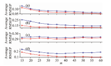
In Fig.6, it is evident that for each transfer method, including CCA-ICE, DS, PDS and SST, at different numbers of m, the RMSEP values of ER are lower than those of KS. Among the four calibration transfer methods, CCA-ICE can generate low prediction errors. CCA-ICE transfers the informative components extracted by the partial least squares (PLS) model. Moreover, the backward refinement can further reduce the errors in a prediction set. For DS and SST, with increasing m, RMSEP values of KS display a decreasing trend, while ER’ s values remains nearly constant. This implies that ER can select key samples for calibration transfer through DS and SST with low errors. In Fig.6(c), although the errors of PDS obtained by KS are larger than those of CCA-ICE, DS and SST, ER can reduce prediction errors by refining the samples.
 | Fig.6 Average RMSEP of corn dataset at different values of m under the transfer set generated by KS (blue line) and ER (red line), respectively (a): CCA-ICE; (b): DS; (c): PDS; (d): SST |
A new transfer set refinement method ER was proposed based on MPA. Initially, ER generated several subsets for the calibration transfer. Subsequently, the average errors of subsets containing this sample were obtained for each sample.
Finally, samples with low average errors were selected as the refined transfer set. The corn dataset was used to test the proposed method. The results indicated that the calibration transfer methods, including CCA-ICE, DS, PDS and SST could reduce prediction errors. Hence, ER can effectively refine the transfer set in calibration transfer.
| [1] |
|
| [2] |
|
| [3] |
|
| [4] |
|
| [5] |
|
| [6] |
|
| [7] |
|
| [8] |
|
| [9] |
|
| [10] |
|
| [11] |
|
| [12] |
|
| [13] |
|
| [14] |
|
| [15] |
|