
加权SPXYE(WSPXYE)算法及其在近红外光谱模型转移中的应用
[郑开逸1  , 封韬
, 封韬1 , 张文1 , 黄晓玮1 , 李志华1 , 张迪1 , 石吉勇1 , Yoshinori Marunaka2 , 邹小波1, * ]
, 封韬]
|
|


样本选择是模型转移的重要组成部分, 其目的是在主光谱和从光谱中选择合适的样本, 建立二者的转移模型, 使得从光谱的预测样本能通过转移模型校正成类似于主光谱的样本, 进而用主光谱的模型直接预测其浓度。 目前, 常用的样本选择算法有: Kennard-Stone 法 (KS法), SPXY法和SPXYE法。 根据上述算法的特点, 提出了一种新的样本选择方法: 加权SPXYE法(WSPXYE法), 进而将其用于选择合适的转移集样本。 WSPXYE同样先计算样本间的距离, 其距离有三个部分组成: 光谱( X)之间的归一化距离 dxs, 浓度( y)之间的归一化距离 dys, 以及校正误差( e)之间的归一化距离 des。 其加权代数和 dwspxye= αdxs+ βdys+(1- α- β) des即为WSPXYE距离。 计算了WSPXYE距离之后, 可以根据其距离选择距离较大的样本作为转移集样本。 WSPXYE是Kennard-Stone法(KS法), SPXY法和SPXYE法的推广, 而KS法( α=1, β=0)、 SPXY法( α=0.5, β=0.5)以及SPXYE法( α=0.333, β=0.333)则是WSPXYE法的特例。 直接校正法(DS)、 有信息成分提取-典型相关分析法(CCA-ICE)作为模型转移算法验证了WSPXYE方法的效果。 结果显示, 与KS法、 SPXY法以及SPXYE法相比, WSPXYE法可以通过调节参数, 选择合适的样本, 获得较低的误差。
, FENG Tao
Biography: ZHENG Kai-yi, (1983-), associate researcher, School of Food and Biological Engineering, Jiangsu University e-mail: kaiyizhengjsu@126.com
Selecting samples in the transfer set is also important in calibration transfer. The purpose of selecting samples in the transfer set is selecting standard samples of both primary and secondary spectra with the same concentrations. After that, the transfer model between primary and secondary spectra can be generated. Finally, the prediction set of secondary spectra can be corrected by transfer model and estimated by the model generated by primary spectra. The commonly used sample selection methods include Kennard-Stone (KS), SPXY and SPXYE methods. Based on the features of those methods, a new sample selection method called weighted SPXYE (WSPXYE) was proposed and applied in transfer set selection. The WSPXYE defines the distance between each paired samples in advance, which is composed of the normalized distances between spectra ( dxs), concentration ( dys) and errors ( des). The weighted sum of the former three distances can set as the WSPXYE distance: dwspxye= αdxs+ βdys+(1- α- β) des. After obtaining dwspxye, the samples with large values of dwspxye, can be selected as transfer set. WSPXYE is the generalization on KS, SPXY and SPXYE methods, while KS, SPXY and SPXYE methods are special cases of WSPXYE with the weights of α and β set as 1 and 0; 0.5 and 0.5 and 0.333 and 0.333, respectively. Two calibration transfer methods, including direct standardization (DS) and canonical correlation analysis combined with informative component extraction (CCA-ICE) has been applied to testing the transfer set selected by WSPXYE. Results showed that WSPXYE could choose proper weights to select good transfer samples to achieve low errors in both validation and prediction sets.
The near-infrared spectra (NIR) have been widely used in pharmaceutical[1], environmental[2] and agricultural[3] researches, because of non-destructive testing, easy operation and fast analysis. As an indirect analysis method, the feasible models of NIR should be constructed in advance, including partial least squares (PLS)[4] and principal component regression (PCR)[5]. Although those linear models have a strong ability in NIR spectra analysis, the reliable model calibrated by one batch of spectra cannot be applied commonly to another batch of spectra, due to baseline drift, wavelength drift and absorbance fluctuations. The problem can be solved by constructing many models each corresponding to one batch of spectra. However, these models may be impractical, and the work of building many models is time-consuming. Thus, calibration transfer can be used as an alternative solution to this problem.
In a pair of spectra batches in calibration transfer, the samples used to construct models are called primary spectra, while the uncalibrated samples only using the model of primary spectra are called secondary spectra.In recent years, many calibration transfer models have been proposed, including DS[6, 7, 8], PDS[9, 10, 11], CCA[12, 13], SEPA[14, 15], CTWM[16], TEAM[17], CT-VPdtw[18], MWFFT[19], and others. Among the many methods proposed, canonical correlation analysis combined with informative component extraction (CCA-ICE)[20] has shown good results for calibration transfer.
In addition to calibration transfer models, the methods of sample selection for transfer set are also important. Nowadays, sample selection methods like Kennard-Stone (KS)[21], SPXY[22] and SPXYE[23] have been proposed and widely used in calibration transfer. All these methods focus on the distances between the values of x, y and calibration errors (e). According to our conjecture, the distances of x, y and e may have different importance for sample selection, and thus, the distances of x, y and e should be assigned as different weights for sample selection. Therefore, in this paper, weighted SPXYE (WSPXYE) was proposed to adjust the weights of x, y and e distances. Meanwhile, WSPXYE was also adopted for sample selection in calibration transfer.
The primary and secondary spectra are symbolized as matrix A and B, respectively. The transfer and calibration sets of spectra A are respectively assigned as At and Ac while the transfer, validation and prediction sets of spectra B are designated as Bt, Bv and Bp, respectively. And y symbolizes sample concentrations. At can be obtained from Ac by WSPXYE method. Meanwhile, the samples of spectra B with the same concentrations of At are assigned as Bt.
Similar to SPXYE[23], the distances of x, y and e from the calibration set of primary spectra with n samples all can be shown as follows
Here, dx(p, q), dy(p, q) and de(p, q) are the distances of samples in x, y and e, respectively. In order to let all weights of the above distances located between 0 and 1, the above distances should be treated as follows
After defining the treated distances of x, y and e, WSPXYE can be shown as follows
Here, α and β are the weights of dxt(p, q) and dyt(p, q), respectively. Meanwhile, in order to balance the weights of dxt(p, q), dyt(p, q) and det(p, q), the weight of det(p, q) can be set as 1-α -β . Thus, the sum of weights of the former three parts is fixed as one. Moreover, in order to make the three weights non-negative, α and β should meet the following conditions:
Inequation (10) can be simplified as
Obviously, KS (α =1, β =0), SPXY (α =β =0.5) and SPXYE (α =β =0.333) are all special cases of WSPXYE. Moreover, by merging the methods of KS, SPXY and SPXYE, WSPXYE can also use the parameters including α and β to adjust the weights of three distances for sample selection. Thus, the sample selection method of WSPXYE is the generalization on KS, SPXY and SPXYE.
Similar to KS and SPXY methods, WSPXYE also selects samples from the calibration set of primary spectra. The procedure of WSPXYE selecting samples from the calibration set with the size of n can be described as follows:
(1) Define the parameters including α , β and the number (m, m< n) of samples selected in transfer set. Meanwhile, two sets should be defined in advance, including Se with selected samples and Su with unselected samples. Obviously, in the beginning, Se is null set and Su is Ac.
(2) Compute the distance (dwspxye) between any two paired samples in Su. Then, find two samples (s1 and s2) with largest dwspxye. After that, allocate them in Se, and remove them from Su.
(3) Compute the dwspxye between any two paired samples belonging to Su and Se, respectively. Choose the sample in Su with the maximum dwspxye. Then, allocate it as s3 in Se and remove it from Su.
(4) Repeat step (3) m-3 times to select the remaining m-3 samples from Su to Se.
(5) Finally, the selected m samples in Se can be assigned as At. Then, the samples of spectra B with the same concentration as that of At are assigned as Bt. Thus, At and Bt can be applied to calibration transfer.
The corn datasets obtained from http://www.eigenvector.com/data/Corn/index.html contain three batches of spectra named as m5, mp5 and mp6, respectively. In these three batches of spectra, each one contains 80 samples with a range of 1 100~2 498 nm and 700 data points. Among the three batches of spectra, mp6 was set as primary spectra, while mp5 and m5 as secondary spectra, respectively. Then, the values of oil were set as y. After that, the values of y were sorted in ascending order, and the middle one of each five contiguous samples was set aside; the residual 64 samples were assigned as calibration set. Meanwhile, in the 16 samples, the first and second samples of each two contiguous ones were set as validation and prediction sets, respectively. Thus, the numbers of samples in both validation and prediction sets are eight. For corn dataset, mp6 was set as primary spectra, while those of m5 and mp5 both as secondary spectra.
By searching, the number of latent variables (l) was set as nine due to the small value of root mean square errors of cross-validation (RMSECV) for calibration set of primary spectra. In addition to l, the number of samples in the transfer set should also be focused on DS. Thus, the RMSEV values at different numbers of m can be computed. Then, at each number of m, under different combinations of α and β , the one with a small value of RMSEV was selected, while the corresponding RMSEV was applied for comparison. The results are shown as follows:
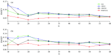
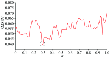
In Fig.1, with m increasing, the RMSEV decreases at first, and after m> 20, the RMSEV keeps nearly constant. Thus, the number of m can be set as 20 for selecting 20 samples for transfer. In addition to m, the weights including α and β should also be researched. In order to obtain the value of α with a low error, the searching range of α can be set between 0 and 1 with a stepwise increase of 0.01. Meanwhile, at each value of α , the RMSEV under different values of β can be obtained, and the minimal one can be chosen as the RMSEV at the fixed α . The results can be shown as follows:
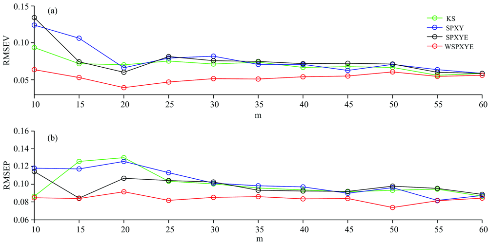 | Fig.1 The RMSEV (plot a) and RMSEP (plot b) of KS, SPXY, SPXYE and WSPXYE methods under different m for mp5 to mp6 transferred by DS |
In Fig.2, it can be shown that at α =0.29, the WSPXYE can achieve small error. Meanwhile, as 0.3 can achieve the same error as that of α =0.29. In order to find the reason behind this phenomenon, the variations of RMSEVV at different β under α =0.29 and 0.3 can be computed and shown as follows:
 | Fig.2 The RMSEV values at different α for mp5 to mp6 transfer by DS |
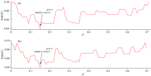
In Fig.3, it can be shown that at α =0.29 and β =0.15 and α =0.3 and β =0.15, the RMSEV can both achieve 0.039 5. The reason may be that the parameter combinations of the former and the latter are close and they generate the same samples in transfer set. Due to α =0.29 and β =0.15 achieving small RMSEV, the weights of x, y and e can be set as 0.29, 0.15 and 0.56, respectively.
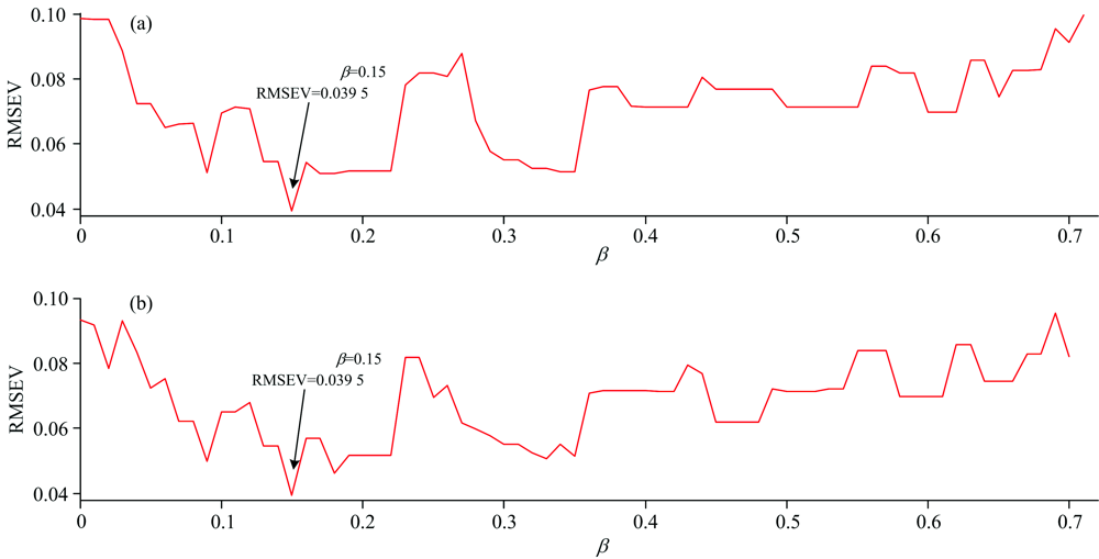 | Fig.3 The RMSEV values at different β for mp5 to mp6 transfer by DS at α =0.29 (plot a) and 0.3 (plot b) |
Moreover, for the purpose of comparison, the KS, SPXY and SPXYE among the commonly used methods were also executed for selecting transfer samples. Meanwhile, the RMSEP of those sample selection methods can also be computed. The results are shown in Table 1.
| Table 1 The RMSEV and RMSEP of mp5 to mp6 transferred by DS |
In Table 1, the WSPXYE can achieve small errors compared with other sample selection methods. In order to further test the effectiveness of WSPXYE, the RMSEV and RMSEP at different m can also be computed. Meanwhile, the errors of KS, SPXY and SPXYE methods can also be obtained for comparison. The results are shown in Fig.1.
In Fig.1, it is interesting that, at each m, both the RMSEV and RMSEP of WSPXYE are less than those of KS, SPXY and SPXYE methods. This can further prove that the WSPXYE can adjust the weights of x, y and e to select better transfer sets than other methods.
In addition to DS, the CCA-ICE as another calibration transfer method can also be used to test the power of WSPXYE. The RMSEV and RMSEP of KS, SPXY, SPXYE and WSPXYE at different m can be listed as follows:
Similar to Fig.1, it can be shown that, at each m in Fig.4, the WSPXYE can generate smaller RMSEV and RMSEP values, compared with the other three methods. Thus, it can be concluded that the WSPXYE selects better samples to obtain good transfer results for mp5 to mp6.
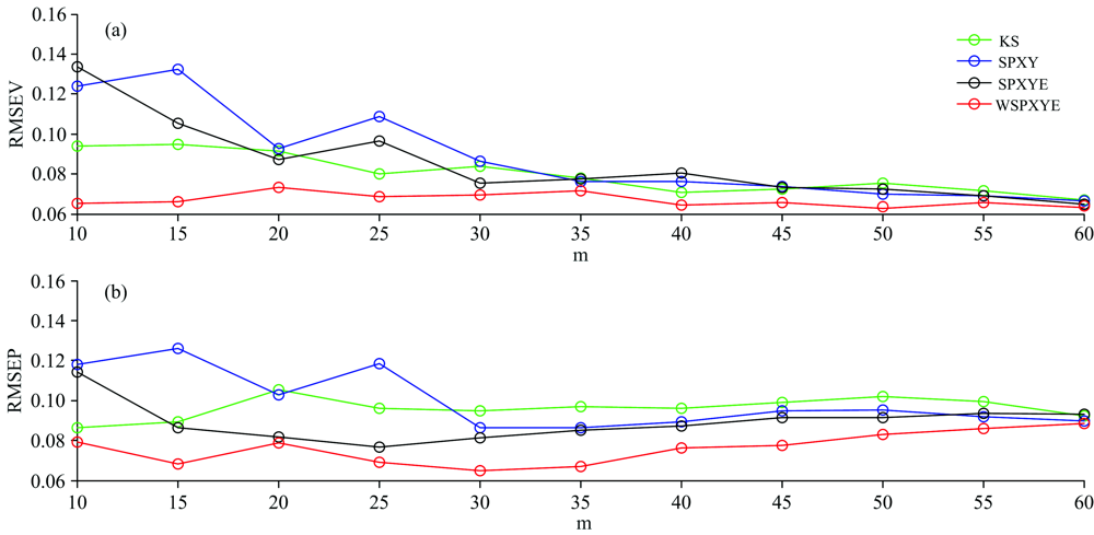 | Fig.4 The RMSEV (plot a) and RMSEP (plot b) of KS, SPXY, SPXYE and WSPXYE methods under different m for mp5 to mp6 transferred by CCA-ICE |
For m5 to mp6, the DS and CCA-ICE can be applied to testing the effect of WSPXYE. In the meantime, other sample selection methods including KS, SPXY and WSPXY, can be applied for comparison. The corresponding RMSEV and RMSEP values at different numbers of transfer sets can be shown as follows:
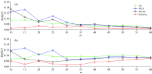
In plots a and b, at each m, the samples selected by WSPXYE and transferred by DS can obtain low errors in both validation and prediction sets. In plot c and d, except for m=15, the WSPXYE can still obtain low errors in both validation and prediction sets. Moreover, at m=15, the RMSEP of WSPXYE is higher than that of SPXYE but still lower than those of KS and SPXY. In the meantime, the root means square error of whole samples in both validation and prediction sets are 0.076 4 (KS), 0.112 (SPXY), 0.080 4 (SPXYE) and 0.064 7 (WSPXYE), respectively. Thus, WSPXYE can still obtain low estimation errors for CCA-ICE. Therefore, WSPXYE can achieve good results compared with those of KS, SPXY and SPXYE methods for m5 to mp6.
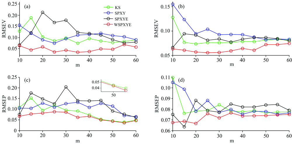 | Fig.5 The RMSEV (plot a: DS; plot c: CCA-ICE) and RMSEP (plot b: DS; plot d: CCA-ICE) of m5 to mp6 |
The WSPXYE was proposed to adjust the weights of x, y and e (errors) as the distances to select transfer set for calibration transfer. The (KS), SPXY and SPXYE methods are the special cases of WSPXYE with the weights of x, y and e as 1, 0 and 0 (KS); 0.5, 0.5 and 0 (SPXY); and 0.333, 0.333 and 0.333 (SPXYE), respectively. Two calibration transfer methods including CCA-ICE and direct standardization DS, were applied to testing the WSPXYE methods. The results showed that WSPXYE could adjust the weights to select proper transfer samples and achieve low prediction errors in both validation and prediction sets.
| [1] |
|
| [2] |
|
| [3] |
|
| [4] |
|
| [5] |
|
| [6] |
|
| [7] |
|
| [8] |
|
| [9] |
|
| [10] |
|
| [11] |
|
| [12] |
|
| [13] |
|
| [14] |
|
| [15] |
|
| [16] |
|
| [17] |
|
| [18] |
|
| [19] |
|
| [20] |
|
| [21] |
|
| [22] |
|
| [23] |
|