基于改进谱聚类的重叠绿苹果识别方法

引用本文

李大华, 赵辉, 于晓. 基于改进谱聚类的重叠绿苹果识别方法[J]. 光谱学与光谱分析, 2019,39(9): 2974-2981.
LI Da-hua, ZHAO Hui, YU Xiao. Overlapping Green Apple Recognition Based on Improved Spectral Clustering[J]. Spectroscopy and Spectral Analysis, 2019,39(9): 2974-2981.
Doi:10.3964/j.issn.1000-0593(2019)09-2974-08 复制到剪切板

Permissions

《光谱学与光谱分析》期刊社所有

基于改进谱聚类的重叠绿苹果识别方法

李大华¹, 赵辉^2,^*, 于晓³

1. 天津大学电气自动化与信息工程学院, 天津 300072

2. 天津农学院工程技术学院, 天津 300384

3. 天津理工大学电气电子工程学院, 天津 300384

*通讯联系人

收稿日期: 2018-07-27 接受日期: 2019-01-05

摘要

水果的可见光谱目标识别是实现农业自动化采摘至关重要的一步。在水果识别的过程中, 由于重叠和遮挡的影响使得目标识别困难, 识别率不高。本文针对自然环境中果实重叠的识别问题, 利用谱聚类算法对图像进行分割, 然后使用随机霍夫变换实现果实的识别和定位。针对传统算法运算复杂度高, 运算速度慢的问题, 本文提出了基于均值漂移和稀疏矩阵原理的改进谱聚类算法。首先使用均值漂移算法对图像进行预分割, 均值漂移是一种用于密度梯度的无参估计法。该算法实质是一种迭代, 先计算出偏移量, 根据偏移量移动点, 如此反复, 直到偏移量为零即收敛到一点为止。利用均值漂移算法除去大多数的背景像素, 为减少谱聚类算法的计算量做准备。然后提取预分割图像的有用信息即图像中像素对之间相似度的描述, 将提取的图像特征信息映射到稀疏矩阵中, 并使用K-means算法将其分类。得到最终的分类结果, 实现对预处理图像的再次分割。然后恢复图像分割区域的颜色, 使用彩色向量梯度提取边缘轮廓, 对得到的轮廓图像使用随机霍夫变换, 并在检测过程中设置半径参数的范围从而进一步加快算法的运行速度。经过检测可以得到目标的圆心坐标和半径, 从而实现重叠绿苹果的识别。降低了谱聚类的数据处理量, 提高了算法的运行速度。经过试验分析和算法对比, 该算法得到较高的重合度95.41%, 较低的误差率4.59%和误检率3.05%。

关键词: 均值漂移; 稀疏矩阵; 谱聚类; 随机霍夫变换; 目标定位

中图分类号:TP317.4 文献标志码:A

Overlapping Green Apple Recognition Based on Improved Spectral Clustering

LI Da-hua¹, ZHAO Hui^2,^*, YU Xiao³

1. School of Electrical and Information Engineering, Tianjin University, Tianjin 300072, China

2. School of Engineering and Technology, Tianjin Agricultural University, Tianjin 300384, China

3. School of Electrical and Electronic Engineering, Tianjin University of Technology, Tianjin 300384, China

*Corresponding author e-mail: zhaohui3379@126.com

LI Da-hua, (1978—), associate professor, School of Electrical and Information Engineering, Tianjin University e-mail: lidah2005@163.com

Fund:the National Natural Science Foundation of China (61502340), the Natural Science Foundation of Tianjin (18JCQNJC01000)

Abstract

Fruits target recognition is one of the most important steps to realize agricultural automation. In the process of fruit recognition, because of the influence of overlap and occlusion, the target recognition is difficult, and the rate of recognition is not high. The paper uses spectral clustering algorithm to solve the problem of overlapped fruit in natural environment. Then the identification and location of fruit are realized by randomized hough transform. In view of the large number of computation and the slow operation speed of the traditional algorithm, this paper proposes an improved spectral clustering algorithm based on Mean Shift and sparse matrix principle. Firstly, the image is pre-segmented using the mean shift algorithm. Mean shift is a non-parametric estimation method for density gradient. The algorithm is essentially an iteration. Calculate the offset, move the point according to the offset, and repeat the above steps until the offset is zero. Most of the background pixels are removed by mean shift algorithm, and the removing is prepared for reducing the computational complexity of the spectral clustering algorithm. And then the useful information is extracted, which is the description of the similarity between the pairs of pixels in the image, and the extracted image feature information is mapped into a sparse matrix. The K-means algorithm is used to classify it into classes, and the final classification result is obtained to realize the re-segmentation of the reprocessed image. Then the color of the image segmentation area is restored, the edge contour is extracted by using a color vector gradient and the randomized hough transform is used on the resulting contour image, and the radius parameter range during the detection process is set to further accelerate the speed of the algorithm. The center coordinates and radius of the target can be obtained through the detection. Thereby the overlapped green apples are recognized. Finally, the algorithm has the high coincidence degree of 95.41%, the low error rate of 4.59% and the false detection rate of 3.05% through experimental analysis and algorithm comparison, and the algorithm meets the practical application requirements.

Keyword: Mean shift; Sparse matrix; Spectral clustering; Randomized hough transform; Target location

文章图片

Introduction

The accurate identification of occlusion and overlapping targets has become the key problem to be solved urgently in the process of machine picking with the advancement of agricultural automation in China^[1]. In view of the problem of segmentation and recognition of overlapping targets, many scholars at home and abroad have carried out research and achieved certain results^[2]. Xu Yue et al. proposed an algorithm combining the snake model with corner detection method for overlapping apple segmentation, which can identify the overlapping fruit, but the overlapping of multiple fruits is not to be identified effectively^[3].

Arman Arefi et al. divided the overlapped tomatoes by a watershed algorithm. It divides fruit with smaller overlaps, but the large overlap area and multiple fruit overlaps cannot be segmented effectively^[4]. Cong Peisheng et al. used watershed labeling algorithm to realize the segmentation of overlapping cells. The efficiency of the algorithm is high, but the robustness to light is poor^[5]. Xie Zhonghong et al. proposed a method based on the concave point searching and the Hof transform. The location and detection of multiple overlapped peaches are realized, and the correct rate is up to 90%^[6].

A method of overlapping tomatoes recognition based on edge curvature analysis was proposed by Xiang Rong et al. It incorporates threshold segmentation and regression criteria. The edge points of eliminating the curvature anomaly are effectively eliminated, and the recognition rate of 90.9% is achieved^[7]. Miao Zhonghua et al. put forward a combination optimization algorithm of image recognition and boundary segmentation for the object overlap in natural environment, which optimizes the combination of k-means and watershed algorithms. The recognition of overlapping targets can be effectively realized under good natural illumination, but the robustness to light is poor^[8].

In this paper, the traditional spectral clustering algorithm is improved by using the principle of sparse matrix and the mean shift algorithm. The problem of the long running time of NCUT algorithm caused by the large amount of data is solved. After getting the target area, use the color vector gradient for edge detection to get the target contour, and use the improved RHT algorithm to identify the target. And the coordinates of the center point of the target are given to prepare for the next step of the robot.

1 Algorithm

This paper improves the spectral clustering algorithm based on the principle of mean shift and sparse matrix. First, it segments the image by means of mean shift. Then a sparse similarity matrix is established based on the combination of the classification information provided by the pre-segmentation and the color and texture features of the image. Finally, the accurate segmentation of the overlapped fruits is achieved. The specific algorithm flow is shown in Figure 1.

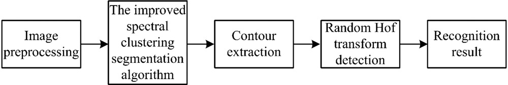	Figure Option View Download New Window
	Fig.1 Algorithm flow chart

1.1 The principle of mean shift algorithm

The mean shift algorithm is proposed by Fukunaga, which is a non-parametric estimation method for density gradient^[9]. The essence of the algorithm is an iteration. First, the offset is calculated and then shift point according to the offset. Repeat the above two steps until the offset is zero, that is, it converges to a point. Mean shift algorithm has a wide range of applications in image segmentation, image smoothing, image tracking and so on. Its basic principles are as follows.

Giving a sample point in a dimensional space x_i(i=1, …, n), the mean shift vector at any sample point x can be defined as

$M_{h} (x) = \frac{1}{k} \sum_{x_{i} \in S_{h}} (x_{i} - x)$ (1)

In which S_h is a high-dimensional sphere region whose radius is h. y is a set of points that satisfy the following relationship

$S_{h} (x) = {y : {(y - x)}^{T} (y - x) \leq h^{2}}$ (2)

k represents the number of points that fall into the area S_h in the sample point.

Kernel function generally satisfies the kernel density estimation K(x)=c_k_,_dk(‖ x‖ ²), in which k(x) is called a core section function. c_k_,_d is a constant, which is the positive number that guarantees the integral of the kernel function K(x) to 1. The kernel function of this paper uses the Gauss kernel function. Let g(x)=-k'(x) and G(x)=c_g_,_dg(‖ x‖ ) to get the extended mean shift vector which is,

$m_{h, G} (x) = \frac{\overset{n}{\sum_{i = 1}} [x_{i} g ({||\frac{x - x_{i}}{h}||}^{2})]}{\overset{n}{\sum_{i = 1}} [g ({||\frac{x - x_{i}}{h}||}^{2})]} - x$ (3)

The mean shift process can be roughly divided into two steps. (1) Calculating m_h_,_G(x). (2) Locating the nuclear window according to it. Let {y_j}(j=1, …, n) be the position sequence of kernel G in the mean shift process. y₁ is the initial position of the nucleus. From the formula (3) we can know that,

$y_{j + 1} = \frac{\overset{n}{\sum_{i = 1}} [x_{i} g ({||\frac{x - x_{i}}{h}||}^{2})]}{\overset{n}{\sum_{i = 1}} [g ({||\frac{x - x_{i}}{h}||}^{2})]} - x$ (4)

y_j records the trail of the shift of the mean shift vector. y_j₊₁≈ y_j when converging. Let x_i(i=1, …, n) be an input vector, z_i is the result of filtering, L_i is the pixel i in the segmented image, then the steps to get the initial segmentation of the image are as follows:

(1) Filtering the input image by means of mean shift vector to get the result z_i of image filtering.

(2) Classifying all point z_i, the starting point converging to the same point is classified as a class. Marking each point and then getting L_i={p|z_i∈ C_p|}。

(3) Eliminating areas of less than m pixels in the marked area L_i.

(4) The area of each classified region (the total number of pixels) is obtained by the histogram. According to the characteristics of the apple image, we set the area threshold, the gray value of the area less than the threshold is set to 0, and the other is set to 1. After obtaining the image, the original image is logically operated with it, and the pre-segmented image can be obtained.

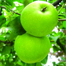
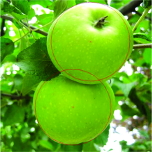
We need to set up the bandwidth vector h=(h_r, h_s), minimum area m and area threshold. The greater the bandwidth is^[10], the more details are lost. Set the wide vector as h=(4, 4) the minimum area as 4, and the area threshold as N/11 in order to preserve more image details. N is the total number of pixels of the image. We enter the test image as shown in figure 2, and the pre-segmented image can be obtained as shown in figure 3.

	Figure Option View Download New Window
	Fig.2 Test image

	Figure Option View Download New Window
	Fig.3 The Pre-segmented image

1.2 Construction of sparse similarity matrix

The traditional spectral clustering algorithm to operate the similarity matrix needs to traverse each element in the matrix. As a result, the amount of calculation is large. We learn from the characteristics of sparse matrices, that is, the storage space is greatly reduced only by storing and processing non zero elements to compute the complexity, but the object to be processed must be a data structure that is compressed and stored by using a specialized sparse matrix^[11].

Based on the advantages of sparse matrix, we improve the shortcomings of the traditional spectral clustering algorithm. We can achieve this goal by constructing a sparse similarity matrix. The generation of the sparse similarity matrix is divided into two parts. The first part is extracting the information feature of the image needed to build the sparse similarity matrix, that is, the description of the similarity between the pixels in the image. In the second part, the extracted image feature information is mapped to the sparse matrix.

1.2.1 Extracting the feature information of the image

The extraction of image feature information, that is, the description of similarity between pixels is the key to accurating segmentation of spectral clustering algorithm. The quality of image segmentation largely depends on the accuracy of similarity between pixels^[12]. The paper makes full use of MS pre-segmentation to get information, and then describesg the similarity between pixels based on the prior information provided by pre-segmentation, the color information and the texture information of images.

$W (i, j) = \max {(W}_{1} (i, j), W_{1} (j, i))$ (5)

$W_{1} (i, j) = W_{c} (i, j) W_{N_{j}} (i)$ (6)

$\begin{array}{l} W_{c} (i, j) = \exp (- \frac{‖ X_{i} - X_{j} ‖^{2}}{σ_{1}} l (i, j)) \times \\ e xp (- \frac{‖ F_{i} - F_{j} ‖^{2}}{σ_{2}} l (i, j)) \end{array}$ (7)

In this paper, the calculation model of similarity is defined as follows:

This paper defines the similarity calculation model as follows. X_i represents the color information of the image. We select the value of H+S-I as the value of the X_i, and F_i is the texture information of the image. According to the analysis before, using the mean value of the four statistical characteristics of the contrast, the two order moments, the entropy and the mean value as the value of F_i. It is the embodiment of the pre- segmentation information of the tag function. The value of!two pixels is 0 when it belongs to the same class in the pre segmentation result, or the value is 1.

$W_{N_{j}}$ (i) is neighborhood influence factors which is set. Using the pre-classified information of the image and the spatial consistency of the image to calculate. Let Sⁱ be the classification of pixel i after pre-segmentation, and j_k represents the pixels in the neighborhood of the j which is N_j.

$W_{N_{j}} (i) = \sum_{N_{j}} \exp (- l (i, j_{k}) λ)$ (8)

Among them, λ is a scale parameter, and the article sets λ =0.01. The definition of W_N(· ) is based on the concept that the more pixels around j are similar to i, the greater the possibility that j and i belongs to the same category. $W_{N_{i}}$ (i) is defined as the neighborhood influence degree of pixel i on j.

Normally W(i, j)≠ W(j, i), W(i, j) indicates the probability of pixel j incorporated into the class S_i. Finally, we take the larger values in W(i, j) and W(j, i) as the similarity between the pixels pair i and j.

1.2.2 The construction of sparse similarity matrix

For the feature information of the extracted image, we need to map the information into the sparse matrix, which requires the following steps:

(1) Calculating the similarity of each pixel point pair in the image as,

$W_{ij} = W (i, j), i = 1, 2, \dots, m, j = 1, 2, \dots, n$ (9)

(2) Translating the similarity matrix into a column matrix U.

$U_{i + (j - 1) \times m} = W_{ij}$ (10)

Getting the characteristic information matrix after merging.

$U = [U_{1}, U_{2}, \dots, U_{N}], N = 1, 2, \dots, m \times n$ (11)

(3) Encoding pixels by the coordinates of the pixels, and the encoding matrix A can be obtained as follows,

$A_{ij} = i + (j - 1) \times m$ (12)

The pixel coding matrix A₁, A₂, …, A_N can be calculated by the upper formula.

(4) Translating the encoding matrix into a one dimensional column matrix S₁, S₂, …, S_N.

$S_{i + (j - 1) \times m} = A_{ij}$ (13)

It is merged to form the abscissa matrix S=[S₁, S₂, …, S_N] of the pixels in the sparse matrix.

(5) Generating the one dimensional column vector

$B_{i} = i$ (14)

Merging the B_i to generate the abscissa matrix D of the pixels in the sparse matrix.

$D = \underset{N}{\underset{︷}{[B_{1}, B_{1}, \dots, B_{1}]}}$ (15)

(6) S, D, U are the three one-dimensional vectors obtained from the upper formula. The coordinates of the feature information matrix in the sparse matrix are stored. Then the sparse similarity matrix can be obtained directly according to the vector assignment.

The complexity of the spectral clustering algorithm is reduced to a through this method. It can effectively reduce the running time of the algorithm while ensuring the accuracy of the spectral clustering algorithm.

(1) The input image I is pre-segmented by means of mean shift algorithm, and the class {L₁, L₂, …, L_h} after the segmentation is obtained.

(2) Calculating W_c(i, j) and $W_{N_{I}}$ (i) according to the prior information provided by pre-segmentation, the color information and the texture features of the image. The neighborhood N_j is set as the 8 neighborhood of the pixel j.

(3) Calculating W₁(i, j) and W₁(j, i) respectively, and taking the maximum as the similarity.

(4) The sparse similarity matrix U is obtained by the obtained adjacency matrix W.

(6) The matrix V is normalized, and the normalized matrix is Y,

$Y_{ij} = \frac{V_{ij}}{\sqrt[]{\sum_{j} V_{ij}}}$ (16)

(7) Regarding the each line of k as a sample is needed to be classified. The k-means algorithm is used to classify it into V class and then getting the final classification results V.

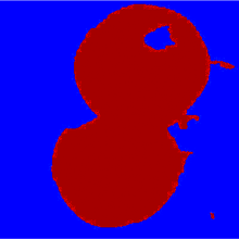
1.3 The Segmentation based on improved spectral clustering algorithm

Selecting the cluster number N=6 according to the experimental experience. Setting the threshold of the target function to 0.06. Inputting the image that is preprocessed and then getting the segmentation results as shown in figure 4.

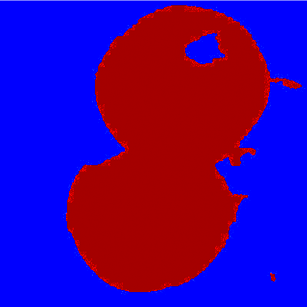	Figure Option View Download New Window
	Fig.4 Clustering results

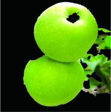
2 Contour extraction and target location

2.1 Contour extraction

First, we restore the segmented image to the color of the target area as shown in figure 5. And then the edge contour is extracted with the color vector gradient.

	Figure Option View Download New Window
	Fig.5 Segmentation results

Setting the of vector Y is the gradient (including the amplitude and direction) of any point (x, y). Let r, g, b be the unit base vectors of the RGB space, we can define the vector as,

$u = \frac{δR}{δx} r + \frac{δG}{δx} g + \frac{δB}{δx} b$ (17)

$v = \frac{δR}{δx} r + \frac{δG}{δx} g + \frac{δB}{δx} b$ (18)

Defining g_xx, g_yy and g_xy as these vectors’ dot product which is shown in the following formula,

$g_{xx} = u \cdot u = u^{T} u = {|\frac{δR}{δx} r|}^{2} + {|\frac{δG}{δx} g|}^{2} + {|\frac{δB}{δx} b|}^{2}$ (19)

$g_{yy} = vv = v^{T} v = {|\frac{δR}{δx} r|}^{2} + {|\frac{δG}{δx} g|}^{2} + {|\frac{δB}{δx} b|}^{2}$ (20)

$g_{xy} = uv = u^{T} v = \frac{δR}{δx} \frac{δR}{δy} + \frac{δG}{δx} \frac{δG}{δy} + \frac{δB}{δx} \frac{δB}{δ y}$ (21)

Using the representation method, the change rate direction θ of the c(x, y) can be given in the following formula

$θ = \frac{1}{2} \arctan [\frac{2 g_{xy}}{(g_{xy} - g_{yy})}]$ (22)

The rate of change value of point (x, y) in the direction of θ is given by the next formula,

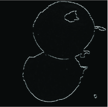
$F (θ) = {\{\frac{1}{2} [(g_{xx} + g_{yy}) + (g_{xx} - g_{yy}) \cos 2 θ + 2 \sin 2 θ]\}}^{\frac{1}{2}}$ (23)

The amplitude of the gradient c(x, y) in the maximum direction θ can be obtained by the upper formula. We use the Sobel operator to calculate the derivation function. Assuming a is the solution of the formula (15), and θ ₀± π /2 is also its solution. But F(θ )=F(θ ± π ), so you only need to calculate θ ∈ [0 π ], that is, there can be two solutions separated by 90° . We calculate the values of two solutions, and one of them is chosen according to the results obtained by the experiment as a solution to the follow-up experiment. The outline of the image is finally shown as shown in figure 6.

	Figure Option View Download New Window
	Fig.6 The ontour of Target area

2.2 Target location

We observe that the outline of the target is interrupted, and there is a small amount of noise. The Hough transform algorithm has good fault tolerance and robustness, and it can also be effectively detected for discontinuous edge contours so we use the algorithm. But the traditional Hough change time is long and the effect is not ideal in actual use^[13]. So we use RHT to detect the target location, and in the process of detection, the range of the radius parameters is set up to speed up the running speed of the algorithm further. The principle of RHT is no longer described in this article. After testing, we can get the center coordinates and radius of the target. The results of the experiment are shown in figure 7.

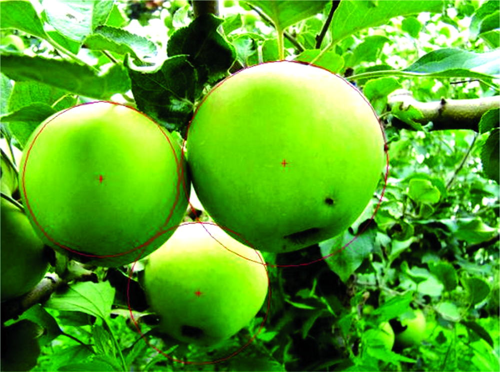
	Figure Option View Download New Window
	Fig.7 The result of the Target location

3 Experimental results and analysis

3.1 Experimental results

In order to verify the effectiveness of the algorithm, we randomly select 20 images (including the image of two overlapped fruits and multiple overlapped fruits) from the test images, and then we verify the algorithm. It is found that the algorithm can not only effectively identify the situation of two overlapped fruits, but also effectively identify the overlap of multiple fruits. The results of the experiment are shown in figure 8 and figure 9.

	Figure Option View Download New Window
	Fig.8 The recognition of multiple overlapped fruits

	Figure Option View Download New Window
	Fig.9 The recognition of two overlapped fruits

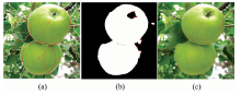
3.2 Analysis of experimental results

Select the experimental pictures randomly. First, use the watershed algorithm to segment the overlapping target area. Then, use Hough to detect the target area after the segmentation, and the experimental results are shown as shown in figure 10 (a). It can be seen from the image that because of the over segmentation caused by the watershed algorithm, which makes the use of Hough transform more interference and can not identify two target regions well.

	Figure Option View Download New Window
	Fig.10 The contrast result of the algorithm (a): Watershed algorithm; (b): Concave point detection algorithm; (c): Proposed algorithm

In the other algorithm, we use an improved spectral clustering algorithm to obtain the target area. Then the concave point is detected and the concave point is detected. Segment the target area according to the concave point and the result of the concave point detection is shown in figure 10 (b). Because of the loss of apple umbilical cord, and the contour of the target area is not smooth enough, there are many concave points detected. Therefore, it is not able to segment two target areas well.

In addition, the traditional NCUT algorithm is used to extract the target area. This algorithm is also carried out in this paper. But during the NCUT clustering, the time of processing a picture has been more than 10 minutes, and the practicability is poor, so this paper does not add the algorithm to the contrast algorithm.

Finally, the experiment is carried out in this paper, and the results are shown as shown in figure 10 (c). It can identify two target areas well. At the same time, the coordinates of the center of the two target areas can also be obtained, which can lay a good foundation for the next step of fruit picking.

In order to obtain the recognition effect of this algorithm further, we randomly select 10 pictures to carry out the experiment, and the actual area(that is the number of pixels we need to recognize) of the images after the experiment are counted. It is marked as A. Detection area (that is the number of pixels the detection circle marked) is marked as B. It can be obtained that overlap area =A∩ B, leakage area=real area-overlap area, misdetected area=detection area-overlap area. And then we define

$Coincidence = \frac{reclosingarea}{realarea} \times 100 %$ (25)

$Segmentationerror = \frac{missingarea}{truearea} \times 100 %$ (26)

$Falsedetectionrate = \frac{falsearea}{truearea} \times 100 %$ (27)

Table 1 can be obtained by statistical calculation.

Table 1 The validity analysis of algorithm

According to the data in Table 1, this algorithm has a high coincidence degree of 95.55%, a lower error rate of 4.45% and a false detection rate of 3.42%. It can meet the requirements of use.

4 Summary

Aiming at the difficulty of overlapping target recognition, which causes the difficulties in realizing agricultural automation, an improved spectral clustering algorithm has been proposed to segment the image in this paper. The improvement of spectral clustering algorithm is based on the principle of mean shift and sparse matrix. First, use the MS to pre-segment the image. A sparse similarity matrix is constructed based on the prior information provided by the pre-segmentation and the color and texture information of the image. It greatly shortens the running time of the algorithm on the basis of the maximum retention of the target area information.

Use the color vector gradient to extract image contour. The target location is realized by using RHT, and the coordinates of the location of the target are obtained. This algorithm can not only identify and locate the overlapped fruit accurately, but also identify and locate the multiple overlapped fruit proofed by the experiment.

Finally, the algorithm is compared with the watershed algorithm, the concave point detection and the traditional NCUT algorithm. Because the running time of the NCUT algorithm is too long, and it is not suitable for the actual picking system. Therefore, the algorithm is not considered in the contrast results. The results show that the algorithm can identify and locate the overlapped fruit effectively. It has a high coincidence degree of 95.55%, a lower segmentation error of 4.45% and a false detection rate of 3.42%. However, in the case of multiple overlapped fruits, this algorithm can identify them, but the segmentation error is large, and there still needs further study.

参考文献

文献列表

[1]	Niu L, Zhou W, Wang D, et al. Multimedia Tools & Applications, 2016. 1. [本文引用:1]
[2]	Song Huaibo, Zhang Chuantong, Pan Jingpeng, et al. Journal of Agricultural Engineering, 2013, (3): 163. [本文引用:1]
[3]	Xu Yue, Li Yinghui, Song Huaibo, et al. Transactions of the Chinese Society of Agricultural Engineering, 2015, 31(1): 196. [本文引用:1]
[4]	Arefi A, Motlagh A M, Mollazade K, et al. Australian Journal of Crop Science, 2011, 5(10): 1144. [本文引用:1]
[5]	Cong Peisheng, Sun Jianzhong, Chinese Journal of Image Graphics, 2006, 11(12): 1781. [本文引用:1]
[6]	Xie Zhonghong, Ji Changying, Guo Xiaoqing, et al. Journal of Agricultural Machinery, 2011, 42(12): 191. [本文引用:1]
[7]	Rong Yingbin, Jiang Huanyu, et al. Journal of Agricultural Machinery, 2012, 43(3): 157. [本文引用:1]
[8]	Wang Dand an, Xu Yue, Song Huaibo, et al. Transactions of the Chinese Society of Agricultural Engineering, 2015, (10): 227. [本文引用:1]
[9]	Petrus B, Haakan L, Eric A. IEEE Transactions on Information Theory, 1975, 21(1): 32. [本文引用:1]
[10]	Tao W, Jin H, Zhang Y. IEEE Transactions on Systems Man & Cybernetics Part B, 2007, 37(5): 1382. [本文引用:1]
[11]	Huo Hua, Feng Boqin. Minicomputer System, 2005, 26(6): 988. [本文引用:1]
[12]	Li Dahua, Shen Mingming, Li Dong, et al. IEEE International Conference on Mechatronics and Automation, 2017. 264. [本文引用:1]
[13]	Ai Lingyu, Kim Eun-Soo. Optics Communications, 2018, 410: 871. [本文引用:1]

2016

0.0

... IntroductionThe accurate identification of occlusion and overlapping targets has become the key problem to be solved urgently in the process of machine picking with the advancement of agricultural automation in China^[1] ...

2013

0.0

... In view of the problem of segmentation and recognition of overlapping targets, many scholars at home and abroad have carried out research and achieved certain results^[2] ...

2015

0.0

... proposed an algorithm combining the snake model with corner detection method for overlapping apple segmentation, which can identify the overlapping fruit, but the overlapping of multiple fruits is not to be identified effectively^[3] ...

2011

0.0

... It divides fruit with smaller overlaps, but the large overlap area and multiple fruit overlaps cannot be segmented effectively^[4] ...

2006

0.0

... The efficiency of the algorithm is high, but the robustness to light is poor^[5] ...

2011

0.0

... The location and detection of multiple overlapped peaches are realized, and the correct rate is up to 90%^[6] ...

2012

0.0

... 9% is achieved^[7] ...

2015

0.0

... The recognition of overlapping targets can be effectively realized under good natural illumination, but the robustness to light is poor^[8] ...

1975

0.0

... 1 The principle of mean shift algorithmThe mean shift algorithm is proposed by Fukunaga, which is a non-parametric estimation method for density gradient^[9] ...

2007

0.0

... The greater the bandwidth is^[10], the more details are lost ...

2005

0.0

... We learn from the characteristics of sparse matrices, that is, the storage space is greatly reduced only by storing and processing non zero elements to compute the complexity, but the object to be processed must be a data structure that is compressed and stored by using a specialized sparse matrix^[11] ...

2017

0.0

... The quality of image segmentation largely depends on the accuracy of similarity between pixels^[12] ...

2018

0.0

... But the traditional Hough change time is long and the effect is not ideal in actual use^[13] ...