


基于法向映射法的二维光纤光谱弯曲校正
[朱海静1  , 邱波
, 邱波1, * , 陈建军2, * , 范晓东1 , 韩博冲1 , 刘园园1 , 魏诗雅1 , 穆永欢1 ]
, 邱波, 陈建军, 范晓东|
|


作者简介: 朱海静, 1991年生, 河北工业大学硕士研究生 E-mail: 691366415@qq.com
二维光纤光谱图是天文望远镜系统中的光谱仪的观测结果, 由此又经过一系列的后续处理, 才能生成普遍意义上的一维光谱。 由于光谱仪和CCD相机的光学畸变, 使得二维光纤光谱图像普遍出现了弯曲现象, 尤其是在光纤两端表现得尤为明显, 这个问题一直以来没有很好的解决办法, 也没有在任何参考文献中看到相关工作。 这种弯曲给后续的抽谱工作造成困扰, 处理不好会很大程度上影响波长定标, 从而影响一维谱的准确性。 给出的一种法向映射法可以对这种二维光纤光谱图的弯曲进行有效的校正。 该法把二光纤光谱图中的每一条光纤光谱进行单独处理。 首先做预处理抽取每根光纤中心线, 然后把该中心线当作光滑曲线求取每个点的法线方向, 以整条中心线的某个点(一般是最凸点)为基点作理想竖直线, 光纤中心线所有点沿自身法线方向投影到这条竖直线上, 从而实现了光纤中心线本身的校直。 因光纤宽度在二维光纤光谱图中一般是7个像素, 因此将光纤中心线向左向右各依次平移3个像素, 分别实现上述流程, 即可得到整条光纤光谱的校直结果。 该法实施过程中有两个问题需要注意: 一个是坐标点的均匀化问题, 一个是像素灰度值的精度保持问题。 坐标点的均匀化问题是由于在该法中使用了法向映射, 从而造成形成后的校直线的点的疏密程度不均匀, 这对后续处理不利。 解决办法是在实际操作中采用三次样条插值的方法进行直线上点的密度均匀化, 保证获得一系列的整数点坐标, 以利于后续的处理。 而像素灰度值的精度保持问题, 在插值计算过程中始终保持像素灰度值的64位高精度数, 最终也得到同样精度的结果, 避免造成像素值损失。 该法实施的最后, 还需要进行头尾一致性的截取, 把延伸出图像高度范围的像素去掉, 仅保留图像范围内的像素点。 如果没有这个过程, 由于光纤本身是有宽度的, 映射出来的直线长短不一, 从而给后续处理造成困难。 实验完整处理了整幅的二维光纤光谱图, 用曲线拟合的方法较好地解决了光纤中心线提取过程中的个别地方的亮度偏差问题, 用法向映射法得到了校直后的二维光谱, 并做了后续的抽谱对比。 在一维谱的抽谱对比中可以看到, 校正前后的谱线差值在有弯曲现象存在的光谱两端变化较为明显。 这个实验结果证明了该方法对光谱的弯曲情况可以完全改善——在两端的变化较大, 在中间的变化很小, 这完全符合观测的基本认知。 不仅如此, 由于像素点的错位和像素值的插值计算, 也会造成流量值叠加的效果发生显著变化。 因此, 通过观察抽谱后的谱线在校正前后的移动情况, 验证了对于特征谱线的波长位置的精确获取具有重要影响。 本文创造性地设计的二维光纤光谱的自动弯曲校正的方法。
, QIU Bo, CHEN Jian-jun, FAN Xiao-dongThe two-dimensional optical fiber spectral images are the observation results of a spectrometer in an astronomical telescope system, and they are followed by a series of post-processing steps to produce the common one-dimensional spectra. Owing to the optical distortion caused by the spectrometer and CCD, obvious bending can be seen from the two-dimensional optical fiber spectral images, especially at both ends of the fibers. So far for this bending problem, there has been no good solution, nor in any reference to see any relevant work. And this kind of bending can cause great troubles to the subsequent spectral lines extraction and other works, which will affect the wavelength calibration to a great extent, as well as the accuracy of the one-dimensional spectrum. In this paper, a normal mapping method has been used to correct the bending phenomenon of the two-dimensional optical fiber spectral images. The method deals with each optical fiber spectrum in the images separately, and corrects the spectrum into vertical straight. The first step is preprocessing, which is to extract each fiber’s centerline. Then the centerline is taken as a smooth curve to obtain the normal direction at each point. The ideal vertical line is based on a point (usually the most salient point) of the whole centerline, and all the points of the optical fiber centerline are projected onto the ideal vertical line along the relevant normal directions, so as to realize the alignment of the optical fiber centerline points, which is the second step. The third step is to handle the whole fiber spectrum. Because the fiber’s width is 7 pixels in the two-dimensional optical fiber spectral image, the fiber’s centerline moves 3 pixels one by one to the left and right, respectively, realizing the above 2 steps and obtaining the straightening result of the whole fiber spectrum. In the whole process, there are two key problems to be noticed: one is the homogenization problem of the coordinate points, and the other is the accuracy maintenance problem of pixels’ values. The uniformity of the sitting punctuation is due to the use of the normal mapping in this method, which results in uneven density of the points after the formation of the alignment, which is unfavorable to the subsequent processing. The solution is to use the cubic spline interpolation method to achieve the density uniformity of the point on the line, to ensure a series of integer coordinates to facilitate the subsequent processing. To maintain the accuracy of pixels’ gray values, the 64-bit high precision number of pixels’ gray values is always kept in the process of the interpolation calculation. At the end of the implementation of the method, it is necessary to intercept both of the two ends of the spectrum to keep the end-to-end consistency, removing the pixels extending out of the height range of the image, and retaining only the pixel points in the image range. If without this process, the mapped vertical lines are different in length, so that causing difficulties in subsequent processing. This paper deals with the two-dimensional optical fiber spectral images, solves the problem of brightness deviation in the process of extracting optical fiber centerlines by using curve fitting method, obtains the corrected two-dimensional spectra after straightening, and makes a follow-up comparison between the one-dimensional spectra. In the comparison, it can be seen that the spectral line differences before and after correction are more obvious than those of the spectra at both ends of the curve. The experimental results show that this method can completely improve the bending of the spectra. It can be seen that the changes at both ends are large and the changes in the middle are very small, which accords with the basic understanding of the observation. Furthermore, due to the dislocation of pixels and the interpolation of pixels’ values, the effect of the superposition of the pixels’ values changes significantly. Therefore, by observing the movement of the spectral lines after the calibration, it is proved that this method has an important influence on the precise acquisition of the wavelength positions of the characteristic spectral lines. This paper creatively designs the method of automatic bending correction of two-dimensional optical fiber spectra and verifies the validity of the method by experiments.
二维光纤光谱数据是目标信号经过望远镜系统后得到的, 其中镜面系统、 焦面系统、 光谱仪系统、 CCD相机等各环节会在一定程度上影响光谱的形态, 使得二维光纤光谱发生较为明显的弯曲[1, 2]。 如图1所示, 图中有250条光纤色散形成的光谱, 有较明显的弯曲形变, 尤其在图像两侧边缘部分[3]。 目前常用的解决办法是在一维抽谱和后续的处理过程中通过和灯谱比对来减轻其影响, 但若能将这些弯曲光谱校正成竖直光谱, 可使后续处理大大简化, 从而有效提高工作效率[4, 5]。 目前此方向的研究并未见诸历史文献。 通过分析二维光纤光谱图的特点, 有针对性地提出法向映射法对其进行校正。
 | 图1 二维光纤光谱图Fig.1 Two-dimension spectrogram |
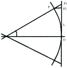
如图2所示, 发生弯曲形变的光纤光谱可看作一段曲率变化的弧OP, 把P点沿着法线方向投射到理想直线上的P1点, 以此为基础提出法向映射校正算法。 此算法是先将二维光纤光谱图像分解开来, 针对某一根光纤的中心坐标弯曲情况进行校正, 然后对一幅图像中的所有光纤光谱逐一处理, 最后整合成新的校正后的光谱。
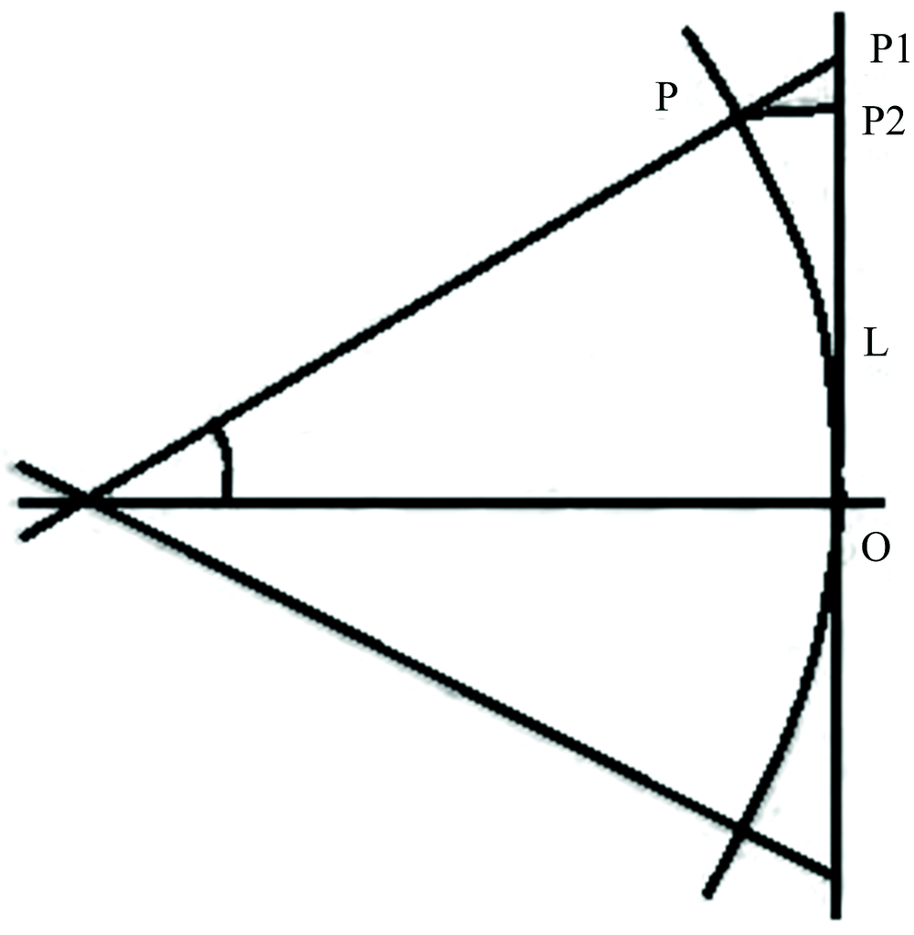 | 图2 法向映射算法原理Fig.2 Principle of normal mapping algorithm |
针对某一根光纤的处理, 法向映射校正算法的基本思路是: 将一段光纤中心曲线上的点逐一求微分, 沿着其法线方向映射到邻近的一条理想直线上。 具体实施如图2所示, P点作为原始光纤上的点, L为待投射的理想直线, 由微分求得P点处的斜率, 对应求其法线斜率及方程, 延长法线与L交于点P1, 即认为P1是P点在理想直线上的映射点。 根据这种方法, 可将光纤中心曲线上任一点映射至直线上。 通过观察可知, 原始光纤若保持纵坐标不变, 水平投影至P2点可保证直线上点疏密一致, 但这种投影并不能反映真实的物理状态; 而法向映射至P1点时, 会造成数据疏密不均, 且纵坐标范围变大, 这个问题可以通过边缘处理及插值运算来改善[6]。
在二维光纤光谱图像中, 按照统计规律, 两根相邻光纤的中心位置大约相差16个像素, 有效的光谱宽度可认为是7~8个像素。 图3(b)显示了光谱的流量曲线。 一般可认为该曲线的最高点对应的横坐标即为光纤中心点坐标。 二维光纤光谱图像预处理就是采用追迹方法找到每根光纤光谱的所有中心点坐标, 经曲线拟合形成整条的光纤中心线, 再以中心线为对象进一步分析讨论。
因天光光谱不考虑宇宙射线及系统噪声的影响, 信噪比高, 因此以二维天光光谱为实验对象, 更易于处理[7]。 实有图像为4 160× 4 136大小的数据矩阵, 理论上分布着250根光谱。 天光光谱图像中, 相邻两光纤之间的灰度值很小, 光谱轨迹所在位置处灰度值很大; 且认为光纤中心处最为明亮, 为灰度峰值, 灰度分布形如高斯函数, 如图3(b)所示。
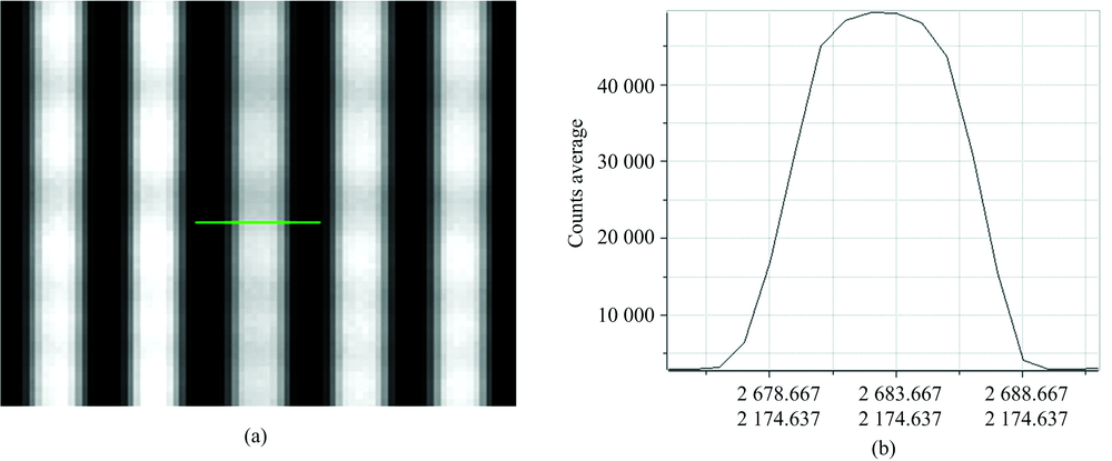 | 图3 光纤光谱宽度示意图 (a): 光纤光谱图像; (b): 光纤某截面由左至右的流量曲线Fig.3 Schematic diagram of spectral width (a): Spectrogram; (b): The flow curve for a section of the optical fiber from left to right |
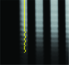
图3(a)中图像横纵向分别为空间方向和波长方向。 对光纤中心进行定位时, 首先取某特定波长处的一行(即固定纵坐标), 定位出该行在空间方向中所有灰度的峰值位置(见图4); 然后依次取各个峰的波长值(横坐标); 重复前两步, 找出全图所有的峰值点, 即可得大致的光纤中心线。
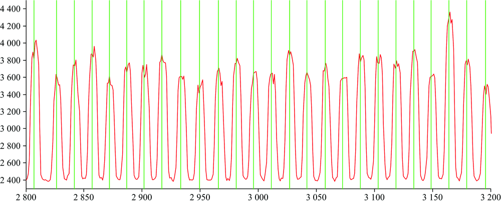 | 图4 光谱图某行的灰度值曲线及峰值定位Fig.4 The gray value curve and peaks’ positions of a line in a spectrogram |
按照上述方法找到所有光谱的中心线。 取某根光纤中心线所有点的坐标, 将这些点显示在光谱图像中, 结果如图5所示。 可见对中心的定位结果较粗糙, 找到的光纤中心是离散点, 凹凸性无规则变化。 针对这个问题, 对每一根光纤中心的坐标, 采用稳健局部回归法处理异常点, 并进行曲线拟合, 使光纤光谱转化为平滑曲线, 得到其表达式, 为校正工作奠定基础。
 | 图5 峰值法标记光纤光谱中心(局部放大)Fig.5 Peak method marking optical fiber spectrum center line |
对拟合完成后的光纤中心曲线进行逐点处理, 利用微分求取每个点的切线斜率, 由斜率推导出其法线方程。 求得中心线上每一点的法线后, 将其延伸, 与光谱宽度的外边界最凸处所在的横坐标直线相交。
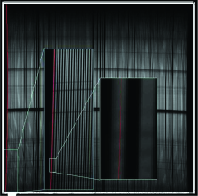
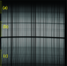
经过映射, 原始中心曲线的坐标位置可一一对应至直线上各点, 并保持灰度不变。 校正结果如图7和图8所示。 其中图8中左侧线表示原数据, 右侧线为映射后的结果(a), (b), (c)分别与图7中区域相对应。 显然, 上下的弯曲得到了明显恢复, 中间部分则与原始数据区别不大, 近于平行。
 | 图6 第一根光谱中心在二维图上的拟合结果Fig.6 Fitting results of the first spectral center on a spectrogram |
 | 图7 三个计算光纤光谱段Fig.7 3 calculation parts of an optical fiber in a spectrogram |
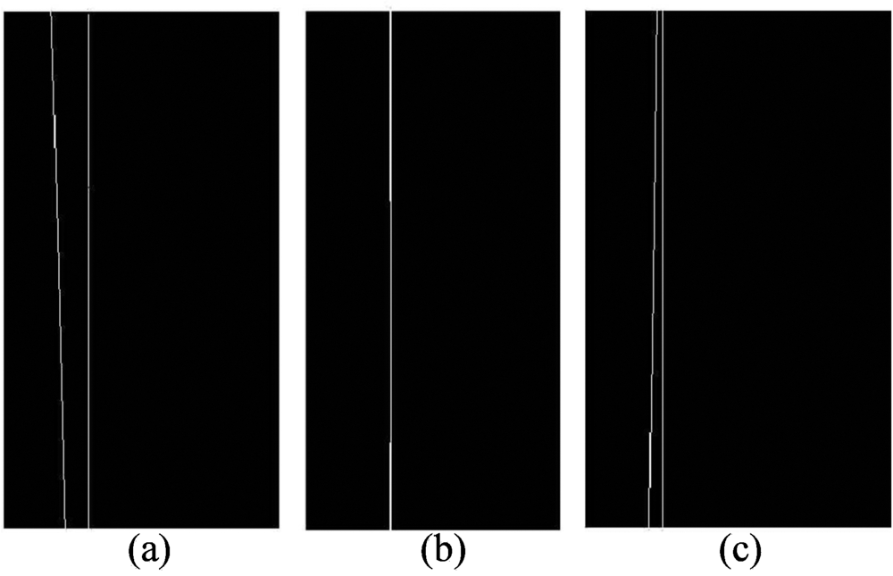 | 图8 光纤中心线校正对比局部放大Fig.8 Partial correction result of a fiber optic center line in Fig.7 |
对光纤中心线两侧的各三列数据分别重复上述过程, 可得校直后的竖直亮带。 由于在法线方向上延伸后更改了横坐标位置, 所以明显地, 所有光谱在波长方向上都变成完全竖直的, 且对坐标点疏密和灰度值分布也做了相应处理, 完全实现了校正的要求。
在得到每一根校正后的光谱后, 为了直观地分析校正前后的光谱变化情况, 选择单条光谱某一波长处的7个像素, 将其灰度沿着空间方向累加, 然后分别对原始光谱数据和校正后的数据在各个波长处进行累加, 得到相应的一维谱线, 并进行对比。 校正前后的数据累加形成的一维谱线如图9所示。
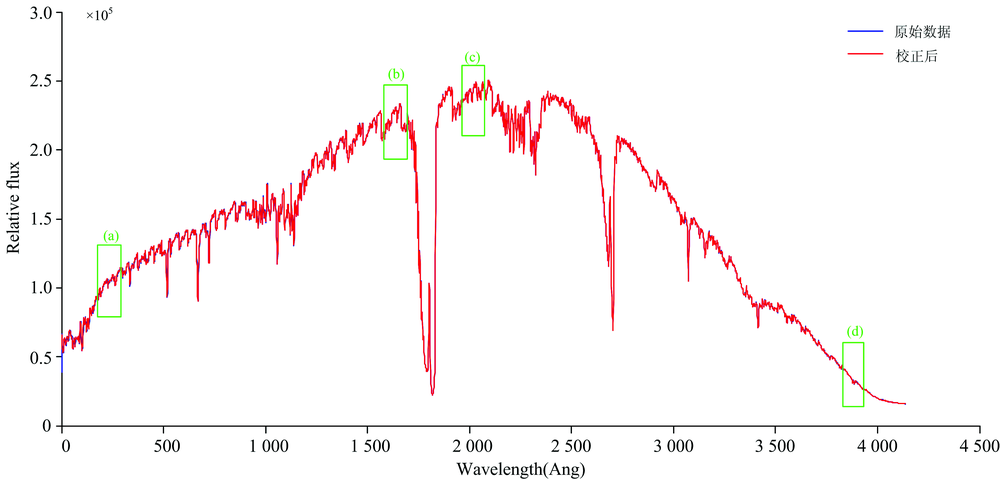 | 图9 校正前后谱线对比图Fig.9 Comparison of spectral lines before and after correction |
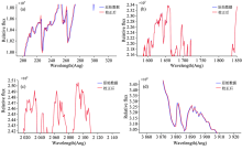
图9中横坐标表示波长方向, 纵坐标表示空间方向上累加后的流量值, 蓝色线为原始光谱累加后的谱线, 红色线为校正后数据的谱线。 由于波长方向数据总量大, 校正后与原数据的横坐标变化量相对整个横轴来说非常小, 导致通过整体谱线不易观察。 通过对图9中的(
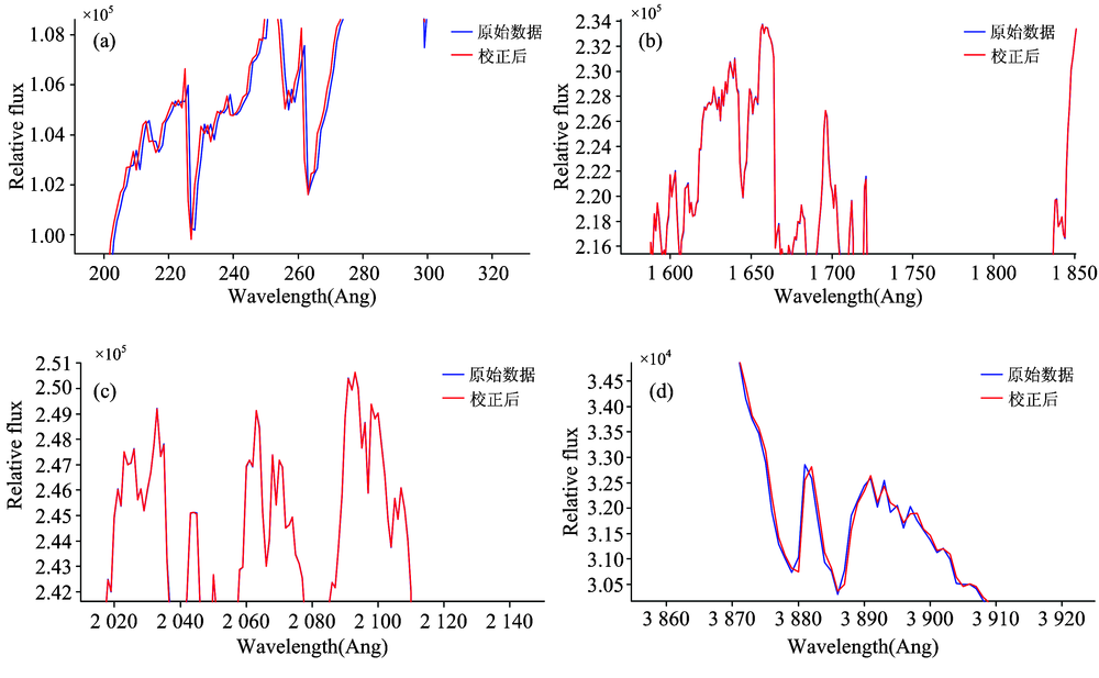 | 图10 校正前后对比(各子图与图9位置对应)Fig.10 Correction comparison (Each sub-graph corresponds to the position of Fig.9) |
由图10可见, 对一维谱线(
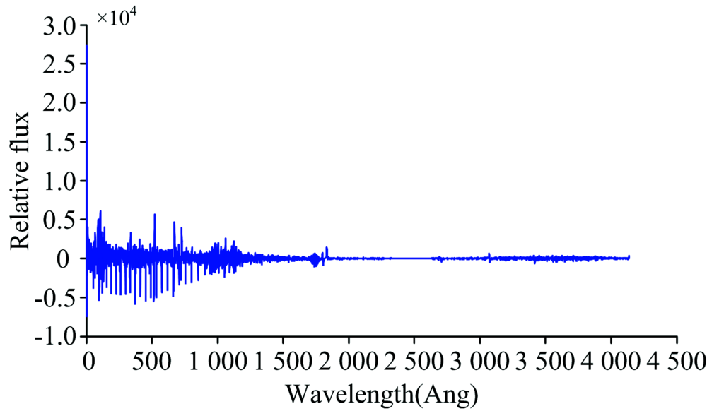 | 图11 校正前后同波长处谱线流量差图Fig.11 Spectral lines’ difference before and after correction |
根据以上分析可知, 校正前后的谱线差值在光谱的两端变化较大。 虽然在屏幕显示和视觉效果上谱线横坐标偏移不便观察, 但结合图11可见校正的效果显著。 如在光谱矩阵的约第500行位置处, 校正前后的灰度差可达到5 000左右。 这在光谱计算和对谱线所含信息的分析中会出现极大的差别。 尤其是对特征谱线的波长位置的精准识别有着重要意义。
将法线映射法应用至整个二维图像中, 再进行整体校正, 就可获得捋直后的二维光纤光谱图。
针对天文二维光纤光谱图像普遍存在弯曲现象进行了校正研究, 提出了法向映射校正算法并进行了实验验证。 实验结果说明, 本方法对抽谱后的特征谱线的波长的精准定位有着重要影响, 而且通过观察可以看到, 特征谱线得到了事实上的增强。
本文率先实现了二维光纤光谱的自动校直处理。 在未来的工作中, 还需在进一步提高方法的准确性方面做出改进。
The authors have declared that no competing interests exist.
| [1] |
|
| [2] |
|
| [3] |
|
| [4] |
|
| [5] |
|
| [6] |
|
| [7] |
|