All commercial reagents used were of analytical grade, Merck (Germany), or Fluka (Switzerland) and were used without further purification.

Recording of the absorption spectra were performed using a UV-Vis spectrophotometer (UV 1700 Pharmasec Shimadzu model) and pH adjustment was performed with Thermo Orion 5-Star pH meter. All measurement were carried out at 25 ℃ using a quartz cuvette of 1.0 cm optical path. Partial least squares and neural network modeling were implemented by MATLAB R2013a software (Math Works).

An aliquot of the 0.4 mol· L^-1 ammonium chloride-acetic acid buffer solution was micro pipetted into a 10-mm quartz cell. Finally, 0.1 mL 7.4× 10^-4 mol· L^-1 eriochrome cyanine R solution was added, and the mixture was briefly agitated (2~5 s). The addition of 0.5 mL sample solution of a metal ion followed, to give a total volume of 2.5 mL. The mixture was then stirred rapidly by a hand-controlled micro-stirrer, and the timer was started. The cell was then placed into the cell holder, and the absorbance was measured against a blank in the range of 400~600 nm. Thus, a total of 32 spectra was collected from a solution, and from such measurements, the spectral data could be arranged into a three-way data matrix. The temperature of the experiments was kept constant at 25 ℃.

A set of standards containing iron(Ⅲ ), aluminum(Ⅲ ) and copper(Ⅱ ) mixtures was prepared at different concentrations, and their spectrophotometric data were measured according to the above procedure. Different chemometrics models were established and were then used to predict the unknown samples.

By convenient dilution of stock solutions, a calibration set of 32 samples were built. Concentrations of the analyte used for the calibration set were in the range 1.0~20.0 ppm. The samples were prepared based on the ratio of water components in the range of each of the three analyte. Standard solutions were prepared in 25 mL volumetric flasks by addition of suitable amounts of each stock solution and diluted by hydrochloric acid to the mark. Also 16 additional samples were prepared similarly to constitute the test set. The UV-Vis spectra of the corresponding solutions were recorded in the same spectral conditions at ambient temperature and the obtained data were used for PLS and ANN modeling.

In this study, a multilayer perception (MLP) feed-forward network was applied for modeling the concentrations Fe³⁺, Al³⁺ and Cu²⁺, schematically shown in Fig.1. The logistic function was used as the activation function in a neural network.

Fig.1

	Figure Option ViewDownloadNew Window
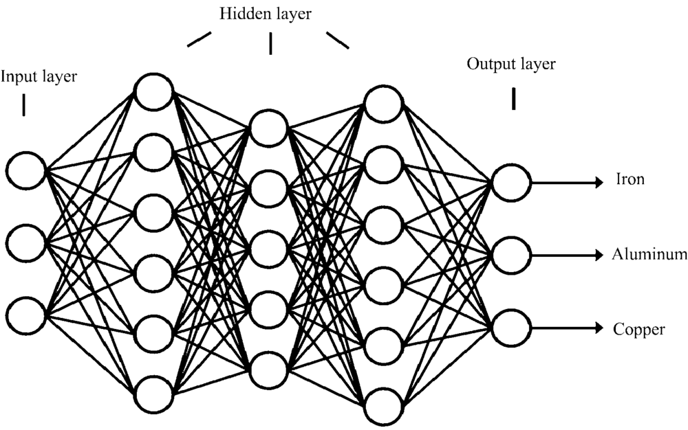	Fig.1 Schematic representation of multi-layer feed-forward neural network architecture

The MLP consists of three types of layers; an input, an output and a hidden layer, each layer contains a number of neurons which operate parallel. These neurons are connected by weights that are modified during the learning phase. Implementing ANN model normally requires a number of steps: data collection, data pre-processing, building the network, training, testing, validation and data post-processing, successively.

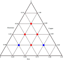
A concentration set of 32 mixture solutions consisting of Fe³⁺-ECR, Al³⁺-ECR and Cu²⁺-ECR in the concentration range of 0.25~1.25, 0.1~0.4 and 0.4~1.2 ppm for Fe³⁺, Al³⁺ and Cu²⁺ in the same solvent were symmetrically prepared from the prepared stock solutions respectively. A ternary diagram was utilized to generate six design points to incorporate different chemical compositions and remove any possibility of factor aliasing (Fig.2). The reason for this is to minimize errors in calibration that may occur during analysis. To check the proposed methods we used an independent validation set consisting of the synthetic mixture solutions of Fe³⁺-ECR, Al³⁺-ECR and Cu²⁺-ECR in the above working concentration ranges.

Spectra from a set of sodium acetate-acetic acid buffer solutions with pH values in the range of 4.0~4.6 were sampled at the reaction time of 300 s (see Fig.3). It can be seen that the different pH conditions did not affect significantly the spectral absorbance of the Fe³⁺-ECR complexes. The absorbance versus pH of the Fe³⁺-ECR, Al³⁺-ECR and Cu²⁺-ECR reactions with the eriochrome cyanine R ligand were also studied at different times with the measurements being recorded at λ _max(Fe(Ⅲ ))=526.8 nm, and λ _max(Al(Ⅲ ))=532.6 nm and λ _max(Cu(Ⅱ ))=519 nm. The kinetic curves for iron(Ⅲ )/ligand aluminum(Ⅲ )/ligand and copper(Ⅱ )/ligand reactions did not change with different pH. Thus, considering all the factors for the pH effects described above, a pH of 4.0 was selected for this work.

Fig.2

	Figure Option ViewDownloadNew Window
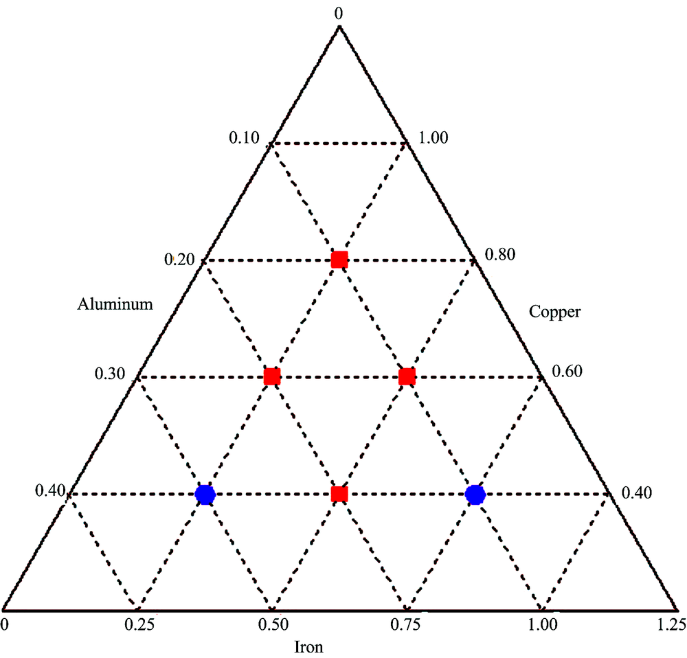	Fig.2 Ternary design diagram. Squares were the calibration data points, and circles were the prediction data points

Fig.3

	Figure Option ViewDownloadNew Window
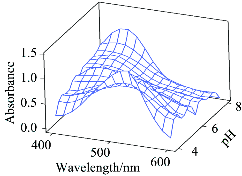	Fig.3 Spectra of Fe3+-ECR complexes at different pH

Fe³⁺-ECR, Al³⁺-ECR and Cu²⁺-ECR ligand complex formation the amount of ECR in order to have the most appropriate, Fe³⁺, Al³⁺ and Cu²⁺ solution pH by adding various volumes of metal solutions ECR ambient pH=4 was adjusted with buffer. Passing to the results obtained with the graphs ligand 12 times more highest absorbance values is reached. According to these results, the most appropriate amount of ligand in the formation of the complex was selected 12 times.

In the first step to developing the PLS-1 model, a calibration set was built with a dataset of 32 samples, in order to take into account the different concentration ratios of analytes and to cover the range usually present in natural water samples.

The full cross validation method suggested by Haaland and Thomas^[24] was used for the accurate selection of the optimum number of factors. This consisted of removing one sample at a time from the calibration step and carrying out the calibration by the remaining samples. The concentration of the one sample removed is expected with the achieved model. This step was repeated for each considered sample. The procedure can be repeated after fixing a different number of factors. Prediction residual error sum of squares (PRESS) was obtained from Eq.(1) and best number of factors was selected in the minimum of PRESS values. In this equation n is the number of samples in the calibration set and C_{i, added} and C_{i, found} are the actual and predicted concentration of analyte in the ith sample, respectively^[25].

PRESS=∑i=1n(Ciadded-Cifound)2(1)

Similarly, the standard error of cross-validation (SEC) can also be defined as

SEC=∑i=1n(Ciadded-Cifound)2n(2)

Where n is the total number of the synthetic mixtures. In order to determine the optimum number of factors, SEC was plotted as a function of different number of factors. The optimum number of factors was obtained to be 2 for Fe³⁺, 5 for Al³⁺ and 6 for Cu²⁺ in which SEC attained the least possible value. Afterwards, the developed PLS-1 model was applied to an independent test set including 16 artificial samples which were not used during calibration. The experimental and found (predicted) concentration of each analyte can be seen in Table 1.

Analytical figures of merit (AFM) are very important to quantify the quality of a given methodology or for method comparison. In multivariate calibration, several AFM have been reported, e.g. selectivity, sensitivity, and limit of detection^{[26, 27, 28]}.

The net analyte signal (NAS) is a new family of multivariate calibration methods that has been defined by Lorber^[26] as the part of a mixture spectrum that is useful for model building. The net analyte signal (NAS) for analyte k ( rk*) is defined as the part of the signal that is orthogonal to the signal of the interferences present in the sample. In general, for inverse calibration methods, it is given by the following equation

rk* =[I-R-k(R-k)+]r=PNAS, kr（3）

where r is the spectrum of a given sample (when r is the spectrum s_k of pure k at unit concentration, Eq. (3) becomes sk*=P_{NAS, k} s_k), I is a J× J unitary matrix, R_-k is a J× A column space spanned by the spectra of all other analytes except k (R_-k+ is the pseudo inverse of R_-k and A is the number of spectral factors used to build the model), and P_{NAS, k} is a J× J projection matrix which projects a given vector onto the NAS space. In factor-based methods such as PCR, PLS and NAS-based methods this latter statement is true only to the extent that the selected factors are representative of the spectra of all other analytes.

Table 1

Table 1

Table 1 Composition of test set and predicted values for Fe3+, Al3+ and Cu2+ by PLS-1 and ANN regression. Concentration values are expressed as ppm Al3+ Fe3+ Cu2+ Actual PLS1 ANN Actual PLS1 ANN Actual PLS1 ANN 0.10 0.06 0.17 0.25 0.20 0.18 0.00 -0.14 -0.23 0.20 0.12 0.28 0.50 0.62 0.40 0.20 0.10 0.25 0.30 0.38 0.26 0.75 0.80 0.85 0.40 0.48 0.38 0.40 0.42 0.28 1.00 1.25 1.36 0.60 0.74 0.54 0.50 0.58 0.49 1.25 1.00 0.98 0.80 0.93 0.69 0.00 0.04 0.25 1.50 1.12 1.25 1.00 1.02 0.84 1.00 1.25 1.35 0.00 -0.26 -0.18 1.20 1.22 1.28 1.20 1.52 0.98 1.75 1.50 1.60 1.30 1.36 1.12 1.40 0.80 1.84 2.00 2.10 1.90 1.40 1.34 1.28 1.60 0.90 1.55 2.25 2.15 2.40 1.50 1.25 1.55 1.80 1.70 1.76 2.50 2.10 2.35 1.60 1.50 1.48 2.00 2.32 2.26 2.75 2.22 2.54 1.70 1.54 1.75 2.20 2.25 1.98 3.00 2.75 2.88 1.80 1.70 1.85 2.40 2.95 2.35 3.25 2.94 3.28 1.90 1.84 1.98 2.60 3.02 2.88 3.50 3.12 3.40 2.00 2.12 2.18 2.80 3.16 2.40 3.75 3.24 3.45 2.10 2.20 2.47

Table 1 Composition of test set and predicted values for Fe3+, Al3+ and Cu2+ by PLS-1 and ANN regression. Concentration values are expressed as ppm

Selectivity (SEL) is an amount, ranging from 0 to 1, of how unique the spectrum of the analyte is, compared with the other species. It requires a part of the total signal that is not lost due to spectral overlap and can be defined by referring to the NAS calculation in a multivariate context:

SEL=‖sk* ‖‖sk‖(4)

Details of the calculations of the NAS in PLS and other Details of the calculations of the NAS in PLS and other multivariate methods are given in Ref.[27]. On the other hand, the sensitivity (SEN) is given by^[29]:

SEN=1‖bk‖(5)

where b_k is the vector of final regression coefficients appropriate for component k, which can be obtained by any multivariate method.

The analytical sensitivity (γ ), which is defined in analogy with multivariate calibration, is the ratio between SEN and the instrumental noise (ε ), according to Eq.(6):

γ=SEN‖ε‖(6)

The value of ‖ ε ‖ may be estimated from the standard deviation in the NAS of several blanks. Concerning the limit of detection, the following simple equation has been proposed for its estimation^[31]:

LOD=3‖ε‖‖sk* ‖(7)

Table 2 shows several estimated FOM for Fe³⁺, Al³⁺ and Cu²⁺ by PLS-1 model.

Table 2

Table 2

Table 2 Analytical figures of merit of the spectrophotometric method by applying PLS-1 for Al3+, Fe3+ and Cu2+ Al3+ Fe3+ Cu2+ Parameter SEL 0.20 0.08 0.04 SEN/(AU* L· mg-1) 0.58 0.29 0.32 γ /(L· mg-1) 22 15 12 LOD/(mg-1· L) 0.029 0.048 * AU is absorbance limit

Table 2 Analytical figures of merit of the spectrophotometric method by applying PLS-1 for Al3+, Fe3+ and Cu2+

In the second part of this work, the spectral data of each analyte was used to develop a neural network model. For this purpose, the network parameters were specified. Among these parameters are; the number of input layers, the number of hidden layers, number of neurons, n each layer, the output layer. In this study several hidden layer with different number of neurons were tested with logistic functions.

It is believed that neural network training can be made more efficient if certain pre-processing steps are performed on the raw input and target data. Randomizing and normalizing data are the most common practices of data pre-processing. Normalization procedure often makes the model more efficient as it prevents the learning algorithm from being confused by the unequal magnitude of different variables and consequently neglecting with the smaller magnitude. The training and testing data sets must be normalized into a range 0.1~0.9. The input and the output data sets were normalized by using following equation:

XN=0.1+0.8(X-Xmin)(Xmax-Xmin)(8)

where X_N is normalized the value of a variable (the network input or the network output), X is a original value of a variable, and X_max and X_min are maximum and minimum original values of the variables, respectively. In order to produce sufficient data for training and testing of the model shown in Figure 1, 32 different standard solutions were prepared using different analyte concentrations and each standard solutions was subjected to spectrophotometric determination. Randomly chosen 800 data pairs from these 1 000 data pairs were used in the training of the neural network, and the rest of the data were used in the testing. The root mean square error values were calculated from following equation to prove quantitatively the accuracy of the testing results of neural network models:

RMS=0.5N-1∑i=1N(X'1-X1)2(9)

where N is the number of testing data and X'₁ is target value.

The developed model which was trained in the previous stage was further simulated by a test set of 16 unknown data. The results obtained by ANN method is listed in Table 2 alongside those predicted by the other method investigated in this work and will be discussed subsequently.

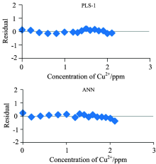
Once the optimal number of factors has been determined, the final calibration may be performed using all the calibration samples with the optimal number of factors. As mentioned earlier, a set of independent test dataset 16 samples which has not been used previously for calibration, was modeled by PLS-1 and ANN methods. The predicted values of each component together with reference values can be seen Table 2. Also, a residual analysis can be carried out by plotting residual vs. the concentration of each analyte. Towards this end, the absolute residual was defined between actual concentration and the predicted value from a model. Figure 4 demonstrates the residual values for the one analyte obtained by PLS-1 and ANN models.

As can be realized in these set of figures, the residual errors committed by ANN method are closely distributed around the zero-order line for all three components. Highest accuracies are obtained for prediction of Fe³⁺ and Cu²⁺ with ANN method with all estimated concentrations close to the reference value. Prediction of Al³⁺ seems to exhibit more deviations than the other components, however, this deviation between experimental and predicted values was mitigated by ANN method in comparison to the PLS-1 regression model.

Table 4 shows a number of important statistical parameters such as the determination coefficient of prediction ( Rpred2, Eq.10), relative error of prediction (REP, Eq. 11) and root mean square error of prediction (RMSEP, Eq.12).

Fig.4

	Figure Option ViewDownloadNew Window
	Fig.4 Residual errors of different methods vs. concentration plots for the one component of test set Rpred2=1-∑i=1n(ci, act-ci, pred)2∑i=1n(ci, act-c)2 (10)

REP%=100×∑i=1n(ci, act-ci, pred)2∑i=1n(ci, act-c)2(11)

RMSEP=∑i=1n(ci, act-ci, pred)2n(12)

where C_{i, act} and C_{i, pred} is the actual and predicted concentration of a component in the ith sample, respectively. C is the mean of actual concentrations in a particular set and n is the number of samples in the test set.

This table also shows the values of the optimal number of factors used for both PLS-1 method and ANN in the calibration set. As can be seen in Table 3, the predictive ability of ANN method was clearly improved after selecting the optimum region of wavelengths. The results also indicate that predictions of PLS-1 and ANN models for Fe³⁺ are in excellent agreement with experimental data, as high R² values of 0.998 9 and 0.998 2 was obtained for these methods, respectively.

Table 3

Table 3

Table 3 Statistical parameters calibration and test set by PLS-1 and ANN regression for three analyte Parameters RMSEP Rpred2 REP/% Al3+ PLS-1 ANN 0.310 0.277 0.965 4 0.934 7 4.46 4.35 Fe3+ PLS-1 ANN 0.532 0.510 0.998 4 0.998 2 2.46 1.80 Cu2+ PLS-1 ANN 0.178 0.138 0.789 9 0.787 6 7.75 8.02

Table 3 Statistical parameters calibration and test set by PLS-1 and ANN regression for three analyte

The data obtained from the methods developed in the light of natural waters Fe³⁺, Cu ²⁺ and Al³⁺’ s determination to UV spectrophotometric primarily as tap water is taken from Sü leyman Demirel University. Representative water behalf affect the results of the experiment natural water sample was filtered twice, then read on the UV spectrophotometer under optimum conditions obtained in the complex formation. Optimization and method development which has been implemented in natural water samples confirmed the results. The recovery result in the application are shown in Table 4. The results are the average of six experiments.

Table 4

Table 4

Table 4 Application of the natural water samples to PLS-1 and ANN validation procedure and the obtained recovery values PLS-1 ANN X̅Fe3+⁃ECR 0.017 4 0.013 2 X̅Al3+⁃ECR 0.005 0 0.004 2 X̅Cu2+-ECR 0.006 4 0.005 6

Table 4 Application of the natural water samples to PLS-1 and ANN validation procedure and the obtained recovery values

The World Health Organization (WHO) and standard values obtained from the literature by Turkish standards are given in Table 5. The test results appear to be obtained within the limits of the chart^{[31, 32]}.

Table 5

Table 5

Table 5 The World Health Organization and the value of TS 266 WHO TS 266 Fe3+ 0.50 0.20 Al3+ 0.10 0.20 Cu2+ 2.00 3.00

Table 5 The World Health Organization and the value of TS 266

Chemometric methods as a result of Fe³⁺, Al³⁺ and Cu²⁺ which is suitable for the analysis of mix and high reproducibility of this method is sensitive and accurate results that showed.