


LIBS技术在污染土壤重金属含量分布测量中的应用
[谷艳红1, 2, 3  , 赵南京
, 赵南京1, 3, * , 马明俊1, 3 , 孟德硕1, 3 , 贾尧1, 3 , 方丽1, 3 , 刘建国1, 3 , 刘文清1, 3 ]
, 赵南京, 马明俊|
|


诱导击穿光谱技术(LIBS)具有实时快速、 多元素同时探测的优势, 并且无需样品预处理, 检测成本低, 是土壤重金属定量分析检测的一种重要分析手段。 将LIBS技术应用于冶炼厂区周围土壤中重金属的含量分布分析研究, 利用Cu, Pb和Cr三种元素的特征谱线强度分析了冶炼厂区周围土壤中Cu, Pb和Cr三种元素的含量分布。 实验结果表明冶炼厂区土壤LIBS光谱中Cu和Pb两种元素的特征谱线强度分布与实际含量分布呈较好的线性关系, 而Cr元素的特征谱线强度分布与实际含量分布相关性较差。 为了提高Cr元素含量分布分析的准确性, 利用CF-LIBS结合Saha方程应用于土壤Cr元素的含量分布分析中。 实验结果表明基于CF-LIBS计算的Cr和Si两种元素含量比值分布与土壤Cr元素的实际含量分布之间具有良好的一致性。 相比于其他的化学分析方法, LIBS技术结合CF-LIBS可以快速的对区域土壤重金属元素的含量分布进行检测, 因此将LIBS技术与CF-LIBS相结合用于土壤重金属的含量分布检测中, 为污染区域的重金属防治提供方向。
, ZHAO Nan-jing, MA Ming-junBiography: GU Yan-hong, (1989—), female, doctoral student, study in Key Laboratory of Environmental Optics & Technology, Anhui Institute of Optics and Fine Mechanics e-mail: yhgu@aiofm.ac.cn
Laser-induced breakdown spectroscopy (LIBS) has become a powerful technology for quantitative analysis of the toxic heavy metals in soils due to its excellent attributes of rapid analysis speed, simultaneous multi-element assay, and low-cost detection with slight sample preparation. In this work, LIBS was applied to analyze the spatial concentration distribution of toxic heavy metals in soils around a smelter. The spectral lines of copper (Cu), lead (Pb) and chromium (Cr) were used to directly analyze the concentration distribution in soils around the smelter. The relevance between the spectral line intensities of Cr and the total concentrations detected by inductively coupled plasma optical emission spectrometry (ICP-OES) was poor. To improve the analysis accuracy, the calibration-free LIBS (CF-LIBS) method combined with Saha equation was used. Compared with the preliminary analysis result of spectral line intensities, the concentration ratios of Cr/Si obtained from CF-LIBS showed a good correlation with the total concentrations. Then, the map of the spatial relative concentration distribution of Cr superposed on the aerial view of the locations was established. Our results demonstrate that LIBS is an efficient rapid method for mapping the spatial contaminated distribution of heavy metal elements and giving us the clear direction to treat heavy metal pollution.
The soilmonitoring has become a severe environmental research due to the heavy metal pollution in soils which is accumulated from the industrial waste, wastewater irrigation, chemical fertilizer, etc. Heavy metals in soils can enter the human body through the food chain to threaten human health. Therefore, there is urgent necessary to develop a real-time and in-situ technique to monitor the toxic heavy metals in soils.
Laser-induced breakdown spectroscopy (LIBS) technique is a real-time, rapid and in situ analytical method for determining the elemental composition with little or no sample preparation[1, 2]. As a procedure of atomic emission spectroscopy, the plasma is generated on the surface of a sample by a highly energetic laser pulse and the emission spectra are detected by a spectrometer. Since each element has the unique emission lines and the intensity of the spectral lines is determined by the concentration of the element, the LIBS spectra can be used for qualitative and quantitative measurementin materials[3, 4, 5]. This technique has beenapplied in a variety of fields in recent years, such as environmental monitoring[6], food security[7], space exploration[8], industrial application[9], etc.
Recently, LIBS has been successfully utilized in spatially-resolved spectrochemical analysis of different experimental materials. Kasier et al.[10] used LIBS technique for measuring the accumulation of lead, magnesium and copper in leaves of sunflower. Galiová et al.[11] utilized LIBS technique for investigating the metal accumulation in vegetal tissues. Lopez-Quintas et al.[12] focused on the use of LIBS technique toanalyze and map the surface topography of stainless steels. Lopez-Quintas et al.[13] applied LIBS technique to map the surface concentration distribution of representative elements and obtained the information about the in-depth distribution of two elementsin different parts of an engine valve. Boué -Bigne[14] utilized LIBS as a micro-analysis technique for mapping the generate elemental concentrationin a large steel sample.
Calibration-Free LIBS (CF-LIBS) is capable of estimating the elemental compositionin unknown target samples without applying calibration curves and a series of certified materials with the matching matrices. This method assumes the stoichiometric ablation, local thermodynamic equilibrium (LTE) and optically thin plasma, which was first proposed by Ciucci et al.[15] To date, CF-LIBS has already been used in many fields for quantitative analysis of materials. Senesi et al.[16] used CF-LIBS to analyze the concentration ratio of Cr/Ti in soil samples, whilea reference soil sample was still been utilized. Pandhija et al.[17] applied CF-LIBS to estimate the concentration of multiple elements in coral skeletons. Kumar et al.[18] focused on the use of CF-LIBS to detect the toxic metals in the sludge of industrial waste water.
In this paper, we report the application of LIBS for detection and quantitation of the accumulation of Cr in soils around a smelter. In order to overcome thestrong influence of matrix effects and inter-element interference on quantitative analysis of Cr with the univariate method, CF-LIBS combined with Saha equation is employedas the semi-quantitative analysis method for the spatial concentration ratio of Cr/Si in soil determination. This study is to investigate the capability of CF-LIBS to rapid evaluate the distribution of toxic heavy metal pollution without calibration samples.
The applied LIBS setup is presented schematically in Fig.1. The LIBS system consists of a Q-switched Nd: YAG laser (Brilliant, Quantel), an Avantes spectrometer, a hemispherical spatial confinement cavity, and a rotary platform. The laser worked at fundamental wavelength of 1 064 nm with a repetition rate of 1 Hz, and the pulse laser beam was focused onto the soil samples perpendicularly using a convex focal lens of 100 mm in focal length. The pulse energy applied in this experiment was 100mJ with pulse duration of 8 ns, and the corresponding laser fluence was 250 J· cm-2. The excited plasma was expanded in the hemispherical spatial confinement cavity which internal diameter was 10 mm to enhance the intensity of the LIBS signal. The cavity had a hole on the upper part which was used to inflate air to blow away the soil dust generated by the experiment. The soil samples were placed onto a rotary platform which was to avoid the pulse laser focusing on the same spot and get better reproducible results. The plasma emission spectrum was transmitted via an optical fiber to the Avantes spectrometer. The spectrometer had three spectrometer channels covering the 200~500 nm spectral range. All the experiments were performed in air at 1atm with a fixed delay time of 1.5 μ s and a 1.05 ms integration time. The instruments were all assembled in a mobile platform portable for field experiment.
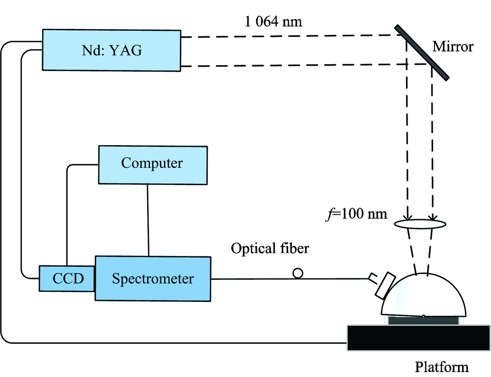 | Fig.1 Schematic diagram of the LIBS experimental setup utilized in soil analysis |
Twelve different soil samples were collected from the open areas around a smelter, Anhui Provence, China by our research group. All of them were located using GPS which can providing two coordinates for each of them, andall of them were taken directly at the surface of the ground. The locations of the sampling points are shown in Fig.2 and they arelabeled from sample 1# to sample 12# in turn, respectively. All of the collectedsoil samples were dried by an electric oven in 100-degree for 10 hours, and then they were finely grinded and sieved through 100-mesh to remove the plant roots. Each 3 g of soil samples was pressed intoa pellet with a diameter of 3 cm and a height of 2.5 mm under 6 MPa pressure by a hydraulic press. The total concentrations of heavy metal elements in soil samples were detected by ICP-OES and the concentrations of several heavy metalsare listed in Table 1.
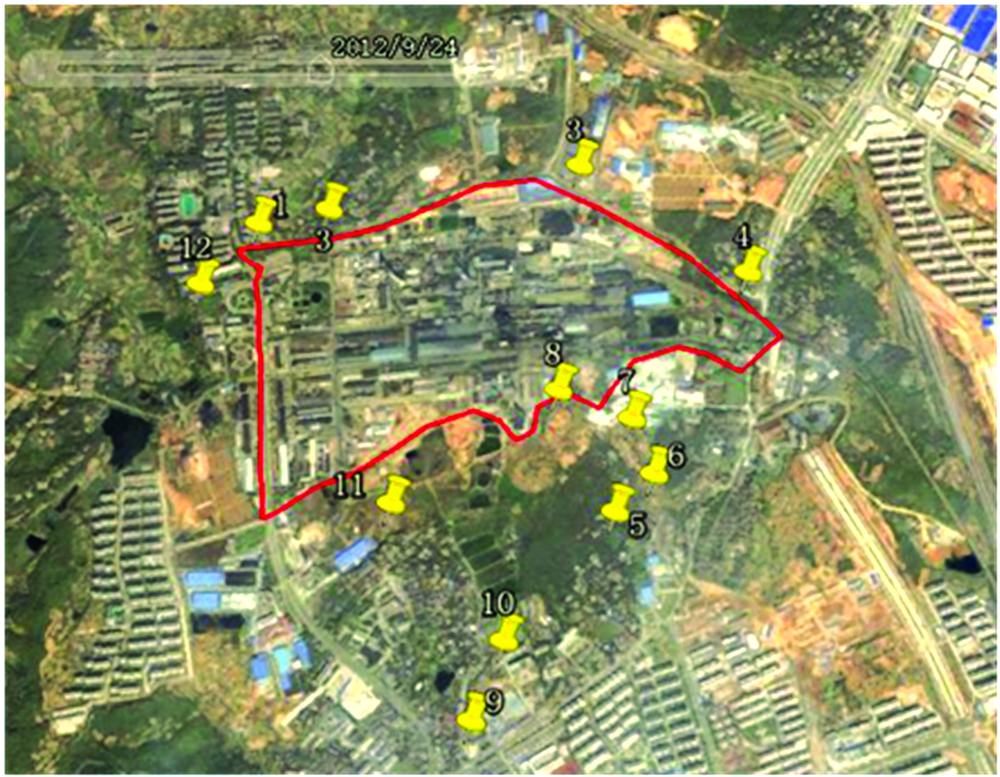 | Fig.2 The locations of the sampling points around the smelter |
| Table 1 Concentrations of heavy metal elementsin soil samples by ICP-OES(mg· kg-1) |
The main purpose of the present work is to evaluate the concentration distribution of heavy metal elements in soil samples around the smelter, in which the prepared soil pellets were detected by the LIBS technique. In order to improve the signal-to-noise ratio, each measured spectrum was the result of an average of 20 laser shots at different locations of the soil pellet. For each sample, ten spectra were detected under the same conditions to reduce the spectral fluctuations and confirm the experimental reproducibility.
Ten measured spectra for each sample were averaged into an analytical spectrum. In laser-generated plasma, the intensities of LIBS signal are proportional to the concentrations of the elements present in the sample, and then, the absolute intensities of Cu Ⅰ : 327.40 nm, Pb Ⅰ : 405.78 nm and Cr Ⅰ : 425.44 nm are used to evaluate the concentrations of Cu, Pb, and Cr. And the intensities of the three spectral lines versus known concentrations are shown in Fig.3.
 | Fig.3 Calibration curves between LIBS intensity and ICP-OES content (a):Cu Ⅰ : 327.40 nm; (b): Pb Ⅰ : 405.78 nm; (c): Cr Ⅰ : 425.44 nm |
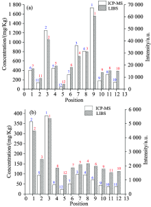
The square correlation coefficient indicates the accuracy of predication, as shown in Fig.3(a) and Fig.3(b), in which the square correlation coefficients of the calibration curves are 0.957 and 0.977. The results are close to 1, which imply that the absolute intensities of Cu Ⅰ : 327.40 nm and Pb Ⅰ : 405.78 nm can indicate the concentrations of Cu and Pb in soils around the smelter. Then we can determine the concentration distribution of Cu and Pb by the LIBS signal. The absolute intensities of the two analysis spectral linesversus the concentrationsat different positions are shown in Fig.4, the numbers on the columns are the content rankings detected by ICP-OES or the intensity rankings detected by LIBS and it is obvious that they have a good correlation in Fig.4(a) and Fig.4(b).
 | Fig.4 LIBS intensities versus the total concentrations by ICP-OES in soil samples (a): Cu Ⅰ :327.40 nm; (b): Pb Ⅰ : 450.78 nm |
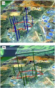
Fig.4 indicates that the concentration distributions of Cu and Pb can be analyzed by LIBS, and they can be intuitively seen by plotting the regional 3-D prismatic map using the gegraph software combined with Google Earth in Fig.5. Then this results implies that LIBS can be an easy and rapid technique for giving us the clear direction to treat heavy metal pollution around the smelter and monitoring soil environmental quality.
 | Fig.5 The map of the spatial concentration distribution of Cu and Pb superposed on the aerial view of the locations around the smelter |
In Fig.3(c), the spectral line of Cr Ⅰ : 425.44 nm was chosen for the analysis of 12 soil samples, the data points versus the total concentrations of Cr are scattered and the square correlation coefficient of the calibration curve is 0.568. As shown in Fig.3(c), the relevance between the spectral line intensities of Cr and the total concentrations detected by ICP-OESis poor. Then the sequenceof spectral line intensities cannot sufficiently accurate represent the concentration distribution of Cr. Fig.6 shows the content ranking of Cr detected by ICP-OES and the intensity ranking of Cr Ⅰ : 425.44 nm detected by LIBS. As shown in Fig.6, the consistency of the two rankings is poor, and the concentration distribution of Cr cannot be directly expressed bythe spectral line intensities of Cr.
 | Fig.6 Quantitative comparison between the spectral line intensities of Cr Ⅰ : 425.44 nm and the known Cr concentrations in soil samples |
Fig.7 shows the representative LIBS spectra recorded in the 422~429 nm spectral region, where it is possible toobserve the two spectral lines of Cr (Cr Ⅰ : 425.44 nm, Cr Ⅰ : 427.48 nm). The contaminated heavy metal element of Cr is trace element in soil samples. In Fig.7, it is clear that other high emission lines (Ca Ⅰ : 422.45 nm, Fe Ⅰ : 425.08 nm, Fe Ⅰ : 426.05 nm, Fe Ⅰ : 427.18 nm, etc) are near them and both two spectral lines of Cr are much lower than them, and it is more likely to have interferences between the spectral lines. For the 12 soil samples, the matrix of them are different and complicated, which can lead different influences on the spectral lines of Cr. The matrix effects and lineinterferences are two severe problems to reduce the measurement accuracy of Cr, which can influencing the spectral profiles and intensities of Cr.
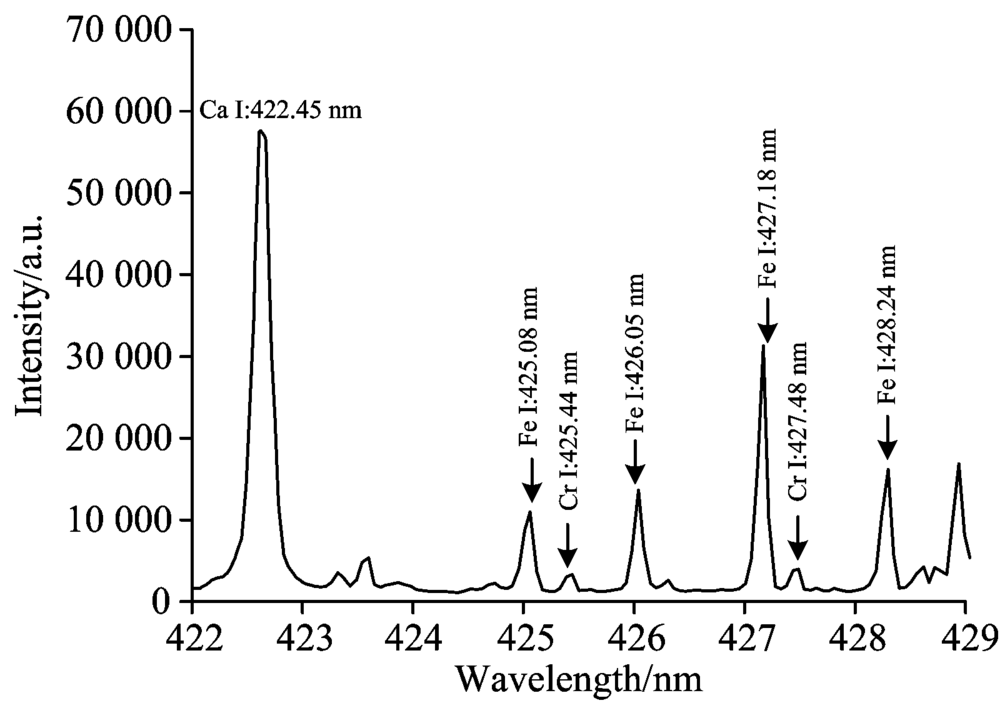 | Fig.7 The typical LIBS spectra in the 422~429 nm wavelength |
The experimental objective of the utilized LIBS setup was to analyze the concentration distribution of Cr in soil samples around the smelter precisely. As mentioned above, the relevance between the spectral line intensities of Cr and the total concentrations detected by ICP-OES is too poor.
Calibration-Free LIBS is a promising quantitative analysis which can avoid the matrix effect without using certified samples and eliminate the use of calibration curve. Assuming the thermodynamic equilibration and the optically thin plasma, the measured elemental line intensity Iij can be proportional to the measured elemental concentration
Where Cs is the atomic concentration of the measured element, F is an experimental parameter, gi is the degeneracy factor of state i, Aij is transition probability, Ei is the transition energy of the upper lever, kb is the Boltzmann constant, T is the electron temperature, and U(T) is the partition function. If wetake logarithm on both sides of the equation 1, the equation can be described by
The spectral lines of ions are not considered in the above equitation, the number density of ions can be calculated by Saha equation
where h is the planck constant, me is the electron mass, and Eion is the ionization energy of neutrals. To improve the accuracy of the concentration analysis, the intensities of the spectral ions emission lines can be calculated by Saha-Boltzmann equation
where Eii is the energy of the upper state of transition of ions. For optically thin plasma in thermodynamic equilibration, the combination of Eq.(2) and Eq.(4) gives
After the iteration of the Saha-Boltzmann equitation, the atomic concentration of the measured element Cs can be described by straight intercept qs of the Saha-Boltzmann equitation. The number density of neutral of singly ionized atoms can be calculated from Eq.(3), and if the plasma is under LTE conditions, the atoms and the ions ratio of a species in the plasma equals the atomic concentration and the ionic concentration ratio in the measured sample.
Besides, the total concentration of the measured elementcan be described by
For estimating the concentration distribution of chromium in soil samples around the smelter, the CF-LIBS procedure has been employed. However, considering the complex matrix of soil samples, it is hard to use the normalization relation on the concentrations of all the elements in the sample. The element-particle ratio combined with CF-LIBS were used to calculate the concentration distribution of chromium in soil samples. For this paper, the soil samples were collected from the same smelter, and the concentrations of dominant element Si in soil samples were assumed as the same. To eliminate the influence of the experimental parameter, the relative concentration of Cr can be calculated by Eq. (8)
where
 | Fig.8 The flow diagram of the calculation about the spatial concentration distribution. |
In the present study, the electron density of Ne is calculated from the stark broadening of Al Ⅰ : 309.28 nm for each sample. Fig.9 shows the Lorentzian profile of Al Ⅰ : 309.28 nm in the soil sample number 1# and the electron densityis calculated using Eq.9.
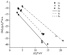
where Δ λ 1/2 is the FWHM of the Lorentzian plot which minuses the influence of instrumental broadening, and w is the electron impact parameter.To evaluate the plasma temperature, a Saha-Boltzmann plot of
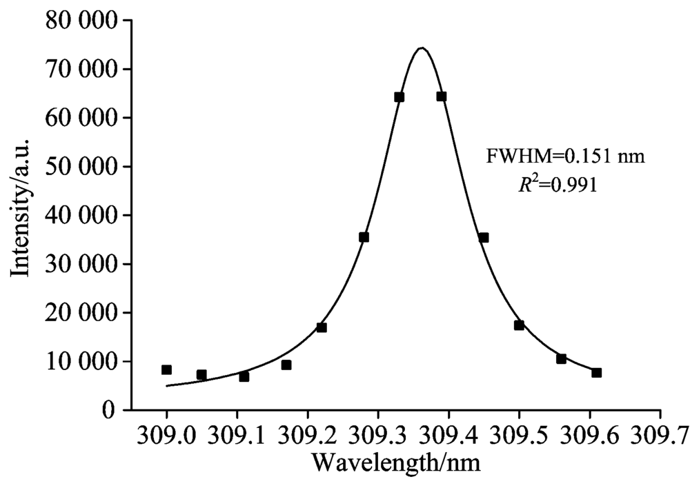 | Fig.9 Lorentzian fitting for the Al line at 309.284 nm |
 | Fig.10 The Saha-Boltzmann plots for elements Fe, Si and Cr in the soil sample |
The values of the plasma temperature and the electron density for twelve soil samples calculating from different experimental data are shown in Table 2. To ensure the existence of LTE, the calculated electron density values which were calculated from Eq.9 should be higher than the lower limit of electron density calculated from Eq.10.
where Δ E is the biggest energy difference between two energy levels in the plasma emission spectrum. The value of T in the conditions of our experiment is 6 097 K, which is the biggest one in Table 2, and the value of Δ E is approximately 6.123 eV. From Eq.10, Ne≥ 2.75× 1016 cm-3 is derived.
| Table 2 Values of plasma temperature and electron density for 12 soil samples |
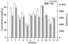
To validate the results obtained by CF-LIBS, the CF-LIBS analysis combined with Saha equation was applied toevaluate the concentration ratio of Cr/Si in soil samples around the smelter and the results are shown in Fig.11. The numbers on the column are the concentration ranking of Cr or the concentration ratio ranking of Cr/Si in 12 soil samples. Fig.11 clearly shows the comparison between the concentration ratio of Cr/Si and the total concentration of Cr in soil samples, and it is obvious thatthey have a good correlation. Then we can approximately determine the concentration distribution of Cr by the concentration ratio of Cr/Si.
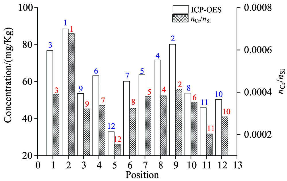 | Fig.11 Semi-quantitative analytical results for the 12 soil samples |
Then using the gegraphs of tware combined with Google Earth to mapping the spatial content ratio distribution of Cr/Si in soil samples around the smelter in Fig.12 and the numbers on the columns are the serial numbers of the sampling locations. The CF-LIBS method combined with Saha equation improved the reliability between LIBS and ICP-OES data. In this way, the entire concentration ratio dataset of Cr/Si can approximately represent the spatial concentration distribution of Cr in soil samples around the smelter directly through the map in Fig.12. This results gained through this experiment show that LIBS technique can therefore be considered as a useful semi-quantitative method and our portable mobile LIBS system can be considered as an available on-site tool for evaluating the soil environmental quality.
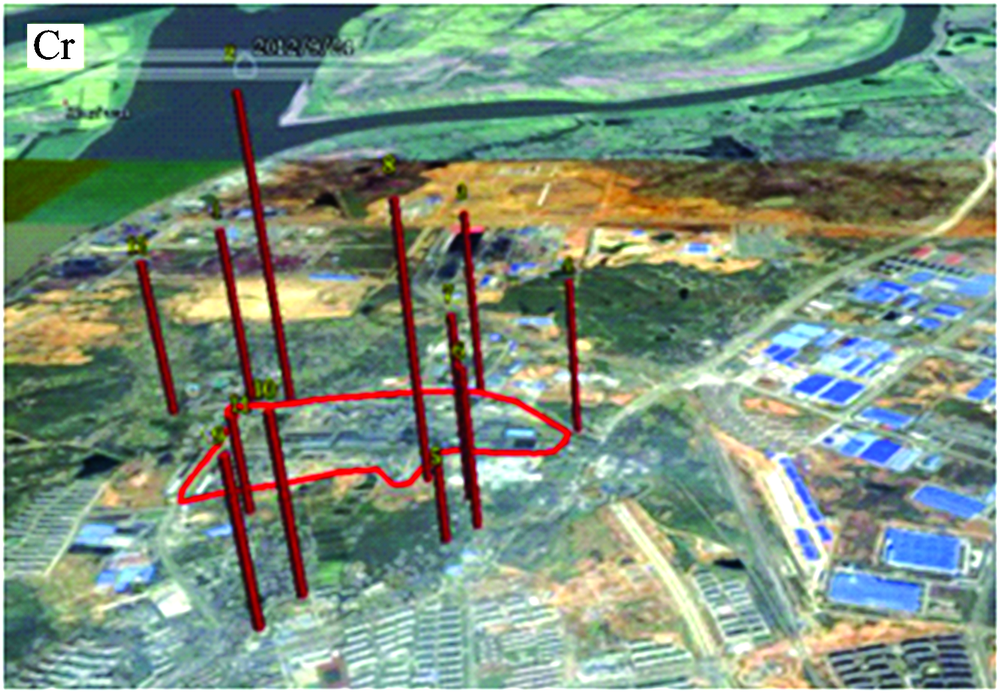 | Fig.12 The map of the spatial concentration ratio distribution of Cr/Sisuperposed on the aerial view of the locations around the smelter. |
In this paper, the capability of LIBS for analyzing the elemental concentration distributions of toxic heavy metalsin contaminated soils around a smelterby a mobile LIBS setup is evaluated. The results of the unvariate quantitative method has been contrasted with the total concentrations detected by ICP-OES. The square correlation coefficient of calibration curves of Cu and Pb are 0.957 and 0.977, and the results show that the concentration distributions of Cu and Pb around the smelter can be measured adequately by LIBS signal.
Considering the issuessuch as the complicated matrix effects, inter-element interference and the fluctuations of experimental conditions, the intensities of Cr Ⅰ : 425.44 nm are not accurate enough to predict the spatial concentration distribution of Cr in soil samples around the smelter. The CF-LIBS method combined with Saha equation has been used to estimate the concentration ratio of Cr/Si and approximately map the spatial concentration distribution of Cr in soil samples around a smelter. The correlation between LIBS signal and ICP-OES data has been improved, and this results indicate that it is feasible to develop LIBS for the analysis of heavy metal contaminated distribution using CF-LIBS method combined with Saha equation. The analytical method employed in this experiment can be extended to other contaminated soils. Moreover, this study indicates that LIBS technique is very useful for directly mapping the spatial contaminated distribution of heavy metals in soils and improves the efficiencies of soil pollution treatment.
The authors have declared that no competing interests exist.
| [1] |
|
| [2] |
|
| [3] |
|
| [4] |
|
| [5] |
|
| [6] |
|
| [7] |
|
| [8] |
|
| [9] |
|
| [10] |
|
| [11] |
|
| [12] |
|
| [13] |
|
| [14] |
|
| [15] |
|
| [16] |
|
| [17] |
|
| [18] |
|